 Newshot
Main
Across many tropical regions, biodiverse old-growth rainforests have been replaced by tree-cash-crop monocultures, including oil palm, rubber, coffee, cacao and timber plantations5. At the same time, both traditional and modern tropical agroforestry systems6—long regarded as reconciling production with ecological sustainability—are being displaced by more intensive agriculture7,8. Such trends in land-use change and land-use intensification pose a substantial threat to the biodiversity and functioning of tropical ecosystems9,10. Quantifying their effects, however, remains challenging owing to the vast effort required to conduct multitrophic inventories of hyperdiverse tropical ecosystems, the often contrasting responses of different taxa, and the scale-dependence of biodiversity11.
The multiple negative effects of land-use change and intensification on tropical biodiversity are increasingly well documented, particularly at the local scale (α-diversity). Previous investigations have shown that α-diversity in tropical agricultural systems is typically substantially lower than in forests, with diminished species diversity linked to declines in ecological functions12,13,14,15. Although protected areas are central to mitigating these negative effects16, the long-term persistence of tropical biodiversity will also depend on conservation beyond reserve boundaries. Designing biodiversity-friendly tropical agricultural mosaic landscapes that sustain regional diversity (γ-diversity) without compromising economic objectives is therefore critical3,8,15. Achieving this goal requires a thorough understanding of how community composition varies among sites (β-diversity)17. β-Diversity arises either from species replacement among sites, with each site hosting a different set of species (turnover), or from species-poorer communities forming subsets of species-richer ones (nestedness)18. Identifying the spatial, environmental and management-related drivers of β-diversity in the context of land-use intensification in hyperdiverse tropical ecosystems may thus guide more effective landscape-scale management19.
An important yet understudied process in this context is biotic homogenization, which has been suggested to be the dominant dynamic shaping species communities and global biodiversity in the Anthropocene20. Biotic homogenization occurs when communities become increasingly similar in composition, often through the loss of specialized, rare or forest-dependent species and their replacement by widespread generalists, including non-native species21. By contrast, biotic differentiation occurs when communities become more dissimilar in species composition, arising from local gains, such as the introduction of non-natives, or from species losses, including the extinction of dominant native species17,22. Patterns of species losses and gains can mask the progressive erosion of biota in formerly forested landscapes, thereby obscuring the true magnitude of the global biodiversity crisis. In heterogeneous agricultural landscapes, differentiation can also result from a variety of semi-natural habitats that support distinct species assemblages. Because homogenization and differentiation can occur simultaneously, understanding their combined dynamics is essential for assessing the full impact of land-use intensification—yet this interplay remains insufficiently explored17,22.
Here we fill this knowledge gap through systematic biodiversity inventories of 24 taxonomic groups across all domains of life, multiple trophic levels, and both aboveground and belowground compartments. Communities were sampled across four different land uses—lowland forests, and three agricultural land uses: low-intensity rubber agroforests (hereafter referred to as jungle rubber) and intensively managed smallholder rubber and oil palm plantations (Fig. 1). Biodiversity and environmental data were collected using a standardized design across 32 sampling plots distributed across 2 distinct landscapes within the smallholder-dominated agricultural tropical lowlands of Jambi Province in Sumatra, Indonesia (Extended Data Fig. 1). This comprehensive dataset builds on a long-term collaborative research programme that has generated detailed taxonomic, functional and trophic information, as well as integrative analyses that link ecological and socio-economic dimensions (Methods). Leveraging this foundation, we provide a novel perspective by investigating the effects of tropical land-use intensification on multitrophic community assemblages at multiple spatial scales. Indonesia combines exceptional biodiversity with one of the world’s highest rates of deforestation, making it a critical frontier of tropical land-use change23,24,25 and a model region for studying land-use trajectories that are increasingly characteristic of smallholder-dominated tropical regions globally.
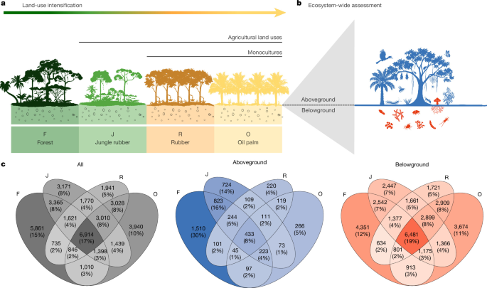
a, The studied land-use intensification gradient ranged from lowland forest (F) to three agricultural land uses of increasing intensity: low-intensity jungle rubber agroforest (J), and intensively managed smallholder rubber (R) and oil palm (O) monocultures. b, Our ecosystem-wide assessment included 24 aboveground and belowground taxonomic groups in Sumatra, Indonesia. c, Land-use effects on the number and proportion of species or microbial OTUs. The shading intensity in the Venn diagrams reflects the number and proportion of species, whether considering all taxa together or separating aboveground and belowground taxonomic groups, with darker shading indicating higher values. Icons courtesy of Ira Taliki (a) and Milena Sampaio (b).
Widespread losses of biodiversity across taxa
We find that the few remaining tropical forests in the region constitute irreplaceable reservoirs of biodiversity. Overall, 5,861 species occurred exclusively in forest (15% of all recorded species in our study; including species, morphospecies and operational taxonomic units (OTUs) or amplicon sequence variants—hereafter referred to as species), including 1,510 aboveground species (30% of all aboveground species) and 4,351 belowground species (12% of all belowground species) (Fig. 1). Forest-dependence was most pronounced for trees, understorey plants and mesostigmatid mites, each with at least 40% of strictly forest-associated species (Extended Data Figs. 2 and 3). These estimates are conservative because our sampling design included three times more agricultural plots than forest plots (Supplementary Figs. 1–3), whereas our sampling effort was equal across all four land-use types. Furthermore, the remaining forests in our study landscapes have faced degradation. Thus, the data probably underestimate the biodiversity potential of intact forests and instead reflect the current trajectory of forest degradation26. Together, these results indicate that a significant proportion of the species pool depends on forests, underscoring the urgency of restoring remaining forest habitats while conserving and preventing further agricultural expansion16,27 and ongoing forest degradation28.
A substantial fraction of biodiversity persisted in agricultural smallholder landscapes: nearly 40% of the recorded species can be considered as forest generalists—that is, species found in both forest and one or more agricultural land uses (15,889 species, 1,966 aboveground and 13,923 belowground taxa). However, almost half of the forest aboveground generalist species (1,966 species) were absent from monocultures and occurred only in forest and jungle rubber (823 species; Fig. 1). At least 60% of aboveground biodiversity (3,057 species) was confined to forest and jungle rubber, and was thus vulnerable to the ongoing loss of (agro)forests13. This trend was especially pronounced for canopy bugs (Hemiptera), hymenopteran parasitoids, spiders and trees (more than 20% of their species were shared only between these two land uses) and bats (40% was shared between these two land uses; Extended Data Fig. 2). Of all belowground species, 19% (6,481 species) were shared across all land uses, with 7% of the species only shared between forest and jungle rubber (2,542 species; Extended Data Fig. 3). The substantial overlap between aboveground forest and jungle rubber communities provides strong empirical evidence that agroforests offer a suitable habitat for a considerably higher number of forest-dependent species than monocultures29,30. Although agroforests cannot replace intact forests, the biodiversity value of traditional agricultural systems, which buffer biodiversity losses in this agricultural landscape, should be recognized. Agroforests also represent a potential leverage point for enhancing biodiversity in human-modified landscapes28, for example, by enriching existing monocultures with native trees3,4.
Overall, land-use intensification drove a marked shift from a species-rich pool of aboveground forest-dependent species to a smaller set of species associated with monocultures. This transition was accompanied by pronounced losses in γ-multidiversity—defined as the average of standardized species richness values across taxonomic groups1 within each land use. Relative to forest (γ-multidiversity = 0.91), γ-multidiversity decreased by 20% in jungle rubber (0.73) and by around 78% in monocultures (0.20) (Fig. 2; Extended Data Fig. 4 for aboveground and belowground γ-multidiversity separately). Thus, our results show clear biodiversity losses with intensification, especially for aboveground species.
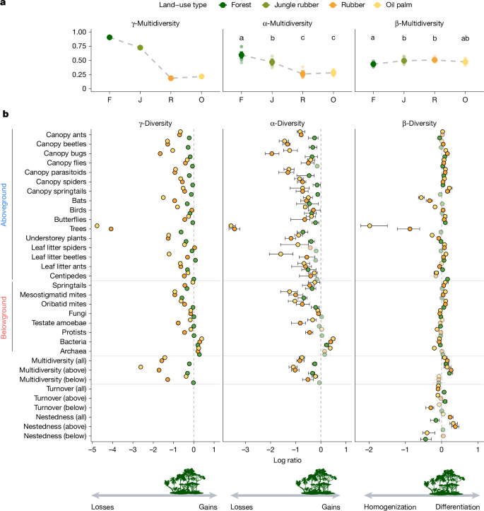
a, Significant effects of land use on α-multidiversity (the average of standardized species richness across taxonomic groups at the plot level; R2 = 0.81, F = 38.68, P < 0.001) and β-multidiversity (the average standardized β-diversity across taxonomic groups per plot based on Jaccard, R2 = 0.30, F = 4.06, P = 0.016) using two-sided analysis of variance (ANOVA) type II. Linear model fits using ggeffect (marginal mean and 95% confidence intervals, n = 32 plots). Letters indicate statistically significant pairwise differences (P < 0.05) based on multiple comparisons of means using Tukey’s contrast, with P values adjusted for the false discovery rate. b, Points and lines (mean and 95% confidence intervals using 10,000 bootstrap replicates) represent log ratio in diversity associated with land-use intensification using forests as a control. Confidence intervals not overlapping zero indicate differences from the forest (coloured points; black confidence intervals; paler colours indicate when the 95% confidence intervals include zero). Negative and positive values indicate decreases (loss of species richness or homogenization) or gains in species richness and differentiation when compared to mean forest values, respectively. For β-multidiversity components, negative and positive values similarly represent decreases or increases in turnover or nestedness relative to forest turnover and nestedness; values for single taxonomic groups are shown in Extended Data Fig. 6.
β-Diversity responses appear idiosyncratic
We hypothesized that land-use intensification would consistently reduce α-diversity across taxa and promote biotic homogenization, such that an agricultural land-use type would harbour more similar communities (lower β-diversity) than forests. By contrast, biotic differentiation occurs when communities become more dissimilar in species composition under an agricultural land use than in forests. To test this hypothesis, we quantified α-diversity as local species richness and α-multidiversity. The α-multidiversity is defined as the average of standardized species richness across taxonomic groups at the plot level1 for each land use using the min–max scaling approach (Methods). To assess changes in community composition within each land use, we quantified β-diversity as aggregated pairwise dissimilarities per plot, and β-multidiversity as the average standardized β-diversity across taxonomic groups per plot using the min–max scaling approach.
We observed a substantial decline in α-multidiversity with land-use intensification (R2 = 0.81, F = 38.68; P < 0.001; Fig. 2, Extended Data Table 1 and Extended Data Figs. 4 and 5), decreasing from 0.59 in forest (95% confidence interval: 0.54–0.65) to 0.47 in jungle rubber (95% confidence interval: 0.42–0.52) and 0.26 and 0.28 in rubber and oil palm plantations, respectively (95% confidence intervals: 0.21–0.32 and 0.23–0.34, respectively; Fig. 2 and Extended Data Table 1). This corresponds to an approximately 50% loss of α-multidiversity from forest to monocultures (Fig. 2). Significant declines relative to forest were observed in 15, 21 and 21 taxonomic groups in jungle rubber, rubber and oil palm plantations, respectively, corresponding to 75%, 94%, and 100% of aboveground taxa, and 38%, 75%, and 63% of belowground taxa (Fig. 2). Trees exhibited the strongest shifts, as they are directly affected by deforestation, planting, and current management practices (herbicide application, manual weeding, liming and fertilizer use), as well as by altered microclimatic and soil-related site conditions in plantations13,30. Such biodiversity losses in monocultures may be partly mitigated locally by improved management31 and diversified, sustainable production systems3,4.
Soil bacteria across agricultural land uses and archaea in oil palm plantations were the only groups in which significant species gains relative to forests were observed (Fig. 2). Species gains for these groups can emerge, for example, as a result of management practices such as liming and fertilization, which increase the soil pH32 and the availability of bio-available nitrogen improving growth conditions for specific bacterial and archaeal taxa33. However, these groups show pronounced shifts in community composition and biotic homogenization (details below; Fig. 2 and Supplementary Fig. 4), highlighting that changes in species richness alone cannot capture the ecosystem-wide effects of land-use intensification.
β-Multidiversity showed only subtle, yet significant, changes across land uses (based on standardized Jaccard; R2 = 0.30, F = 4.06, P = 0.016; Fig. 2 and Extended Data Table 2). This less pronounced multidiversity loss was partly explained by taxon-specific patterns of biotic homogenization or differentiation (Fig. 2). Significant biotic homogenization—lower β-diversity in the agricultural land uses relative to β-diversity in forests—was found in 5, 6 and 9 taxonomic groups in jungle rubber, rubber and oil palm, respectively; whereas 9, 13 and 12 groups showed significant differentiation—higher β-diversity in the agricultural land uses relative to forests. The remaining groups showed neither significant homogenization nor differentiation. Only 10 out of 24 taxonomic groups responded consistently across agricultural systems—either homogenization (understorey plants, fungi and bacteria) or differentiation (canopy bugs, flies, parasitoids, spiders, butterflies, leaf litter beetles and oribatid mites; Fig. 2).
Idiosyncratic responses probably reflect land-use-specific effects on habitats and the interactions between disturbance and environmental heterogeneity19,34 (Supplementary Fig. 5). For example, biotic and abiotic filtering may drive homogenization in tree communities by directly causing the loss of forest specialists through management. Effects can also act indirectly via resource homogenization—for example, through fertilization or homogenization of plant resources in terms of composition and seasonality, impacting niche segregation across trophic and non-trophic interactions. Further indirect effects act via seed dispersal, recruitment, growth and survival34. Similarly, homogenization in soil microbial communities may arise from filtering through shifts in plant–fungal associations35 and from reduced dispersal limitation via passive dispersal36,37,38. By contrast, biotic differentiation can arise from spillover and occasional species, as observed previously in arthropods19 and supported by our results on abundance-based dissimilarity indices for canopy arthropods (Supplementary Results). Biotic homogenization and differentiation can result not only from changes in community composition but also from changes in spatial aggregation, species abundance distributions and individual densities per unit area39. These ecological mechanisms are biologically relevant, modified by land-use intensification and captured by our approach39.
Turnover was the dominant component of β-multidiversity across land uses, ranging from zero in oil palm for trees to 0.93 in rubber for leaf litter spiders. Turnover multidiversity reflects the extent to which sites within the same land use host distinct species assemblages across multiple taxonomic groups. Turnover multidiversity increased in jungle rubber (log ratio: 0.07; 95% confidence interval: 0.02 to 0.11) and decreased in monocultures (log ratio rubber: −0.10; 95% confidence interval: −0.15 to −0.06 and log ratio oil palm: −0.09; 95% confidence interval: −0.13 to −0.05) compared with forest (Fig. 2). Stronger declines in turnover multidiversity were observed in oil palm for aboveground taxa (log ratio: −0.10; 95% confidence interval: −0.15 to −0.07) and in rubber for belowground taxa (log ratio: −0.30; 95% confidence interval: −0.44 to −0.22; Extended Data Fig. 6). Nestedness across land uses ranged from 0.02 in jungle rubber for fungi to 0.48 in rubber for centipedes. Relative to forest, nestedness multidiversity—indicating assemblages in species-poor sites forming subsets of those in species-rich sites within the same land use across taxonomic groups—increased for aboveground taxa in rubber (log ratio: 0.38; 95% confidence interval: 0.27–0.47) and oil palm (log ratio: 0.32; 95% confidence interval: 0.23–0.44) plantations and decreased on belowground taxa in jungle rubber (log ratio: −0.44; 95% confidence interval: −0.58 to −0.28) and oil palm (log ratio: −0.40; 95% confidence interval: −0.52 to −0.18) plantations (Fig. 2 and Extended Data Fig. 6).
Our results reveal that disentangling the components underlying biotic differentiation within each land use is essential; differentiation emerging from nested assemblages has different implications for conservation and landscape management than differentiation emerging from the uniqueness of species assemblages. Distinguishing these processes sharpens our ability to anticipate trajectories of biotic homogenization, including the delayed effects of extinction debt and colonization lags, whereby an apparent differentiation may in fact reflect assemblage simplification before a transition towards homogenization occurs17,19,22. Biotic differentiation can emerge when differences—for example, in local landscape properties—among sites lead to increasing differentiation over time, resulting in homogenization within the same landscape but differentiation among landscapes (landscape divergence hypothesis)40. Weak homogenization or biotic differentiation can also result from higher forest cover in smallholder landscapes; forest cover may guard against homogenization through, for example, edge effects and source-sink dynamics. Smallholder plantations in our study region lie at the deforestation frontier41—other regions that have undergone earlier land-use change may consist of larger, more homogenous, intensively managed industrial plantations (not included in our study). Therefore, higher levels of homogenization and shifts from differentiation to homogenization are expected as smallholders allocate more land to the main crop42 and optimize management and logistics to increase crop profitability8,41,43 and on large-scale industrial plantations. These considerations help to identify points of intervention in existing plantations and in plantations that are entering second and third generations to increase differentiation and promote more sustainable landscapes2,3,4.
Ecosystem-wide impacts of land-use change
Land uses differed markedly in species composition, as shown by the ordination of mean pairwise community dissimilarities aggregated across all taxonomic groups (Fig. 3) and the analyses of similarities (ANOSIM; R = 0.92; P < 0.001). Compositional shifts from forests to monocultures were primarily associated with changes in microclimate and vegetation structure (Fig. 3). These results were corroborated by a multiple factor analysis, which identifies a common structure across two or more data matrices without assuming causal relationships44. The common structure across taxonomic groups and environmental variables aligned with land use (the first dimension explains 18% of the variance and was associated with land-use type), and was mostly driven by compositional shifts in fungi, protists, bacteria, oribatid mites, and canopy spiders and bugs (Supplementary Table 1 and Supplementary Fig. 6). A previous study, using the same plots, shows a compositional shift in terms of a loss of plant symbionts and a gain of pathogenic fungi with land-use intensification35, despite almost no change in fungal richness across land uses. Therefore, understanding compositional shifts in soil communities is highly relevant because they affect ecosystem functioning—for example, via aboveground–belowground interactions and nutrient cycling33,35.
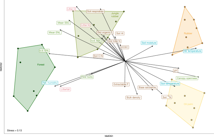
Non-metric multidimensional scaling (NMDS) ordination of mean pairwise dissimilarities (Jaccard index) across plots, aggregated across all 24 taxonomic groups. Polygons delineate land-use types. Vectors indicate environmental variables, grouped by category. The categories are microclimate (blue: air temperature, mean air temperature; rel. humidity, mean relative air humidity (%); soil moisture, mean soil moisture (vol%); soil temperature, mean soil temperature); vegetation (light green: canopy openness; fine roots, fine root productivity; mean ENL, mean effective number of vegetation layers; mean SSC, mean stand structural complexity; s.d. ENL, standard deviation effective number of vegetation layers; and s.d. SSC, standard deviation stand structural complexity); litter (pink: litter C, litter carbon content; litterfall; and litter N, litter nitrogen content); and soil properties (brown: bulk density; ECEC, effective cation exchange capacity; base saturation; extractable P, Bray extractable phosphorus; pH, soil pH; soil 15N, soil 15N natural abundance signature; soil Al, aluminium saturation; soil C:N, soil C:N ratio; soil organic C, soil organic carbon; soil respiration; and soil total N, soil total nitrogen).
Identifying primary drivers of biodiversity change is crucial to landscape management. Studies of β-diversity have often contrasted the roles of ecologically neutral processes with those of niche-based community assembly45,46,47. Strong contributions of geographical distance to β-diversity indicate a prevalence of neutral, dispersal-related processes, whereas strong contributions of environmental variables indicate an important role of habitat filtering48. To disentangle the relative contributions of geographical distance, environmental differences and landscape context to β-diversity, we performed generalized dissimilarity modelling (GDM)49. The GDMs explained substantial variation in β-diversity (>50%) for understorey plants, fungi, bacteria, protists, canopy spiders, beetles, bugs, parasitoids and springtails, as well as trees, archaea, butterflies and oribatid mites (Fig. 4). The variation in pairwise β-diversity was strongly related to environmental variables, particularly vegetation and litter availability, both of which vary with land-use types42. By contrast, geographic distance contributed only weakly to β-diversity for most taxonomic groups (Fig. 4). This suggests a stronger role of habitat filtering, rather than dispersal, in structuring the species assemblages in the landscape mosaic under study.
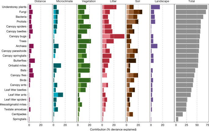
Results from GDM. For each group of environmental variables, principal components were calculated and selected until the cumulative explained variance reached 80%; these components were used as predictors in the GDM. Colour shading denotes individual principal component dimensions. Variable loadings are shown in Extended Data Fig. 7. Model statistics and predictor importance using Monte Carlo sampling with 250 permutations are reported in Supplementary Tables 2 and 3. Landscape context is represented by the mean forest cover within a 200 m concentric buffer surrounding each plot.
The three taxonomic groups with the strongest explanatory power—understorey plants, fungi and bacteria—also exhibited homogenization in the agricultural land uses (Fig. 2). This pattern suggests that homogenization is driven, to a large extent, by deterministic processes associated with land-use-induced changes in the environment, including direct impacts from soil disturbance and fertilization, and indirect effects from the deliberate replacement of forest species with a single, often non-native, target crop, and an alteration of vegetation structure by establishing even-aged structure. Additionally, biotic homogenization is driven by characteristics of the surrounding landscape (Supplementary Table 3). Processes leading to biotic differentiation can also emerge from changes in vegetation structure, as observed in most canopy-dwelling groups. Thus, for many groups, homogenization and differentiation can be linked to drastic changes in habitat structure following land-use intensification30 and in the remaining surrounding forests. Still, biotic differentiation can also be only weakly related to environmental conditions and the surrounding landscape, as for leaf litter spiders, mesostigmatid mites and springtails. Thus, biotic differentiation could be more stochastic and potentially driven by disturbance, legacy effects or meta-population and meta-community dynamics that were not quantified here.
Conclusions
Our results provide detailed insights into how tropical land-use intensification restructures biodiversity through concurrent changes in species richness and community composition. We document pronounced declines in γ- and α-multidiversity from lowland forests to monocultures, driven primarily by aboveground taxa. The diminishing tropical (degraded) forests and traditional agroforestry systems in our study region constitute irreplaceable reservoirs of biodiversity, but their biodiversity is in peril and requires urgent conservation and restoration actions. Divergent responses between aboveground and belowground compartments underscore the need to integrate multiple taxonomic groups spanning body size and mobility. We found no evidence for consistent community homogenization with land-use intensification. Instead, consistent with previous work, we found taxon-specific and seemingly idiosyncratic patterns of both biotic homogenization and differentiation19,20,22,50, but we also revealed a systematic shift from turnover to nestedness in monocultures. Our results call for careful interpretation of spatial patterns of community homogenization and differentiation, as well as long-term monitoring, because homogenization–differentiation trends can be scale-dependent (in line with the landscape divergence hypothesis) and can differ between smallholder and industrial plantations, which are not included in our study. In addition, early stages of assemblage simplification may mask trajectories towards biotic homogenization. Overall, our results demonstrate that land-use intensification alters multidiversity across spatial scales, with ecosystem-wide consequences for biotic communities and their abiotic environment, and suggest that habitat filtering has a stronger role than neutral or dispersal processes. Effective conservation will benefit from recognizing the conservation value of traditional agricultural systems, which, in our study region, buffer the loss of multiple generalist forest species and exhibit high levels of β-diversity. These traditional agricultural systems are currently under pressure from conversion and lie outside the conservation focus and landscape planning. Furthermore, implementing sustainable management practices2,3,4 within conventional monocultures could help mitigate biodiversity losses and promote landscape differentiation in these agricultural landscapes. Differentiation across multiple taxonomic groups should not overshadow the homogenization occurring within key taxonomic groups such as bats, birds, trees and understorey plants. Therefore, there is a growing need to establish conservation priorities for focal taxonomic groups, including tailored landscape-scale solutions to maximize the γ-diversity of forest-associated biodiversity, such as conserving irreplaceable endemic species in this biodiversity hotspot.
Methods
Study region and study design
Our study was conducted in the province of Jambi on the island of Sumatra, Indonesia. This tropical lowland region has undergone extensive land-use changes since the twentieth century and is a showcase of smallholder agriculture in Indonesia13,42. Two sample landscapes, ‘Harapan’ and ‘Bukit Duabelas’ (with loam and clay Acrisol soils, respectively), were selected within Jambi Province. In each landscape, four 50 m × 50 m replicate plots were established in each of the four land-use types common to the region: primary degraded forest (sensu ref. 51), jungle rubber (a traditional agroforestry system established by planting rubber trees inside secondary forest), smallholder monoculture rubber plantation, and smallholder monoculture oil palm plantation—totalling 32 plots. The number of replicate sites per land use is comparable to that of other ecological studies in tropical lowland regions52. Various measurements, such as microclimate, were taken at the plot level. Other measurements, such as most biodiversity sampling, were taken in five permanent 5 m × 5 m subplots established within each plot. All sites were selected in 2012. At this time, rubber plantations were established 7–16 years ago, and oil palm plantations were established 8–15 years ago. For jungle rubber, plots selected contained older non-rubber trees, with individual rubber trees of varying ages not planted in rows13.
Jungle rubber, rubber and oil palm plots were owned and managed by smallholder farmers, whereas the forest plots were located in the Bukit Duabelas National Park and the Harapan Rainforest Restoration concession area (PT REKI). In our study region, smallholders generally do not cultivate food crops alongside the target cash crops examined here, with only a few exceptions8,42,43. Our study’s oil palm plots were on average surrounded by ~13.6% forest and ~61% oil palm plantations within 1 km buffers compared with ~0.45% and ~96% in industrial oil palm plantations, respectively41. Further, our oil palm plots received less herbicide (0.73 l ha−1 year−1) and fertilizer (6.6 kg N ha−1 year−1) compared with industrial oil palm plantations41 (1.12 l ha−1 year−1 and 141 kg N ha−1 year−1). Rubber and oil palm smallholder plantations represent the highest land-use intensity level among the systems included in our study. Yet land-use intensity is even higher in large-scale industrial plantations. More information on the study region, study design, land-use types and management practices of the smallholder systems is provided elsewhere8,13,42. Data compilation in these studies has also served as a basis for our study, but has been substantially expanded in recent years. For example, a multi-taxon perspective was offered in ref. 42 for 3 taxonomic groups, in ref. 13 for 9 taxonomic groups, and in ref. 8 for 14 taxonomic groups.
Species data
We studied 24 different biodiversity indicators distributed from the canopy to the soil, namely: (1) ants (Hymenoptera: Formicidae), (2) beetles (Coleoptera), (3) true bugs (Hemiptera), (4) flies (Diptera)53, (5) parasitoids (parasitoid Hymenoptera), (6) spiders (Araneae), and (7) springtails (Collembola), from the canopy; (8) bats (Chiroptera), (9) birds (Aves), (10) butterflies (Lepidoptera), (11) trees (Tracheophyta), (12) understorey plants (Tracheophyta), (13) spiders, (14) beetles, and (15) ants, from the leaf litter; (16) centipedes (Chilopoda), (17) springtails, (18) mesostigmatid mites (Mesostigmata), and (19) oribatid mites (Oribatida), from the litter and soil; and (20) fungi, (21) testate amoebae, (22) protists, (23) bacteria, and (24) archaea, from the soil (Supplementary Table 4). These biodiversity indicators represent a wide spectrum of taxa, encompassing all domains of life, various trophic levels, and diverse ecological strategies, dispersal abilities and body sizes. This comprehensive dataset builds on a long-term collaborative effort that generated detailed insights into individual taxonomic groups, including species descriptions54,55,56,57,58,59, field guides60,61,62,63 and functional and trophic interactions53,64,65,66—as well as ecosystem-wide analyses and integrative studies linking ecological and socio-economic dimensions8,13,42.
Canopy arthropods
Canopy arthropods (ants, beetles, bugs, flies, parasitoids, spiders and springtails) were collected by canopy fogging in the dry season from May to October 2013. In each of the 32 plots, 3 representative canopy locations were selected, avoiding canopy gaps and overly dense canopies. At each of the 3 locations, 16 rectangular traps (1 m × 1 m) fitted with 100 ml ethanol-filled bottles were suspended from ropes beneath the selected canopies at approximately 1.50 m. 50 ml of DECIS EC 25 (active ingredient: deltamethrine 25 g l−1), dissolved in 4 l of petroleum white oil, was applied to the target canopies from the ground using the Swingtec Swingfog SN 50. In all four land-use systems, target canopies consisted of leaves from different trees. Stunned and dead arthropods were collected from the traps up to 2 h after the complete application of the fogging mixture. Canopy fogging was conducted in the early morning, immediately after sunrise, to minimize air movement that would disperse the fog. This was done only in dry conditions, ensuring that small arthropods would not become trapped in water droplets on leaves and branches. Overall, 372,146 canopy arthropod individuals were collected this way53 and sorted into morphospecies for selected taxa. This study includes data from the following taxa: ants (Hymenoptera: Formicidae) 179 morphospecies67; beetles (Coleoptera) 397 morphospecies in 4 families (Chrysomelidae, Curculionidae, Elateridae and Staphylinidae)68; true bugs (Hemiptera) 301 morphospecies in 2 suborders (Auchenorrhyncha and Heteroptera); flies (Diptera) 483 morphospecies in 2 suborders (Brachycera and Nematocera, including Eudiptera)69; parasitoid wasps (Hymenoptera: “Parasitica”) 1,012 morphospecies in 6 families (Braconidae, Ceraphronidae, Encyrtidae, Eulophidae, Scelionidae and Platygastridae)70; spiders (Araneae) 445 morphospecies71; and springtails (Collembola) 60 morphospecies72. Recorded (morpho-)species across taxa are deposited in the http://ecotaxonomy.org database and in refs. 60,61,62.
Bats
Bats were surveyed using mist nets and harp traps between April and August 2015. We used telescopic aluminium poles to install mist nets with a total length of 48 m, as well as two harp traps (1.35 m × 1.75 m) in presumed bat flyways. Mist nets were 3 m high, with a 19-mm mesh size, and were installed at ground level or up to 3 m high, depending on plot conditions. Each plot was sampled from 17:30 to 22:00 on two consecutive nights, resulting in an average sampling effort of 1,296 m2 of mist net hours. We checked the nets and traps every 15 min until 20:00 and every 30 min thereafter. Harp traps were left on site until and checked the morning after. Captured bats were left in tissue pouches until the nets were closed. Then bat morphology was measured to identify them according to the latest bat species checklist for Sumatra73. We tagged the bats’ nails with nail polish colour codes to identify recaptures and released them afterwards. This study includes data from 20 bat species. In plot HJ3, no individuals were caught (total abundance = 0).
Birds
Birds were sampled with point counts74, as well as automated sound recordings, from May to July 2013. Point counts and automated sound recordings lasted 20 min and were conducted from the centre of each plot between 6:00 and 10:00. The timing of point counts alternated between early and late morning, and all plots were visited three times. The automated sound recorders (SM2+ with two SMX-II microphones, Wildlife Acoustics) were set up at ~2 m height to record at a 44.1 kHz sampling rate in stereo, simultaneously across land-use types; one recording, starting at sunrise, was used for each plot. Point count detections of individuals flying above the canopy were excluded, and unfamiliar bird calls were recorded using a Sennheiser ME-66 directional microphone. The automated sound recordings were uploaded to ecoSound-web, an online platform for ecoacoustics75, for two independent ornithologists to identify all bird calls within an estimated 35 m radius. Only bird species identified by both ornithologists in recordings of each plot were used and subsequently merged with the species list obtained from the point counts. Aural detections were confirmed with cross-checks on the Xeno-Canto online bird call database (https://xeno-canto.org/). This study encompasses data from 114 bird species. For birds, BO1_5 data were unavailable. Therefore, when analyses required non-missing values, imputation was performed by using the average from plots of the same land use within the same landscape (that is, Bukit). However, γ-diversity values for birds may be underestimated.
Butterflies
Butterflies (Lepidoptera: Papilionidae, Pieridae, Lycaneidae and Nymphalidae) were recorded from all 32 study plots in the dry season of 2017 between August and October. Butterflies were collected using sweep netting on three parallel 50-m transects per plot, with two transects on the outer boundaries and the third through the centre. Sweep netting was conducted once in the morning (8:00−11:00) and repeated in the afternoon (13:00−16:00). Except for two voucher specimens per collected species, all butterfly individuals were released on the evening of the sampling day. This study includes data based on butterfly specimens from 219 species76. Recorded morphospecies are deposited in the http://ecotaxonomy.org database and in ref. 63.
Trees and understorey plants
Plant inventories were conducted between February 2013 and August 2014, using different sampling schemes for large trees and vascular understorey plants30. All trees per plot with a diameter of ≥10 cm at a height of 1.3 m were identified. Vascular understorey plants were censused in the five 5 m × 5 m subplots per plot, including all plant individuals, such as terrestrial plants (herbs, shrubs, climbers and juvenile trees) and epiphytes growing up to 3 m above the ground. 281 tree species were present in both censuses (for large trees and understorey plants). To avoid inflating species richness, they were retained only in the matrix that included large trees. Species identification was conducted in the field if possible or otherwise based on field photographs and herbarium specimens deposited at BIOT, BO, GOET, and the herbaria at Jambi University and Harapan Rainforest (acronyms follow Index Herbarium: http://sweetgum.nybg.org/science/ih/). The number of all individuals per species and plot was used for analyses. In total, this study includes 443 tree species and 976 vascular plant species in the understorey.
Leaf litter arthropods (spiders, beetles and ants)
Leaf litter was collected from three of the five subplots within each of the study plots. In each subplot, leaf litter from 1 m2 of ground was sieved using a coarse mesh (width of 2 cm). All macro-invertebrates visible to the naked eye were hand-collected from the sieved samples, stored in 65% ethanol and transported to the laboratory for identification12. Recorded (morpho-)species are deposited in the http://ecotaxonomy.org database. This study includes data on 135 morphospecies of ants, 170 morphospecies of beetles, and spider specimens from 132 morphospecies. For leaf litter spiders and leaf litter beetles, no individuals were detected in plots HO2 and BO4, respectively (total abundance = 0).
Centipedes
Between October and November 2013, random samples were taken from three 5 m × 5 m subplots per plot (a total of 96 samples). Samples were taken at least 2 m from the next tree or dead-wood accumulation. Each sample measured 16 cm × 16 cm and included the complete litter layer and the underlying topsoil to a depth of 5 cm, obtained using a spade. Animals were extracted using heat and stored in 70% ethanol77. This study includes data from 12 morphospecies. In plot BR2, no individuals were detected (total abundance = 0).
Springtails
Samples were taken in October 2013. In each plot, one randomly positioned soil core (16 cm × 16 cm) was taken to a depth of 5 cm in the mineral soil. Litter and soil layers were separated in the field and extracted independently. Animals were extracted by heat for 5–10 days until the substrate was completely dry78, collected in dimethyleneglycol–water solution (1:1) and stored in 70% ethanol79. This study includes data from 58 morphospecies.
Mesostigmatid mites and oribatid mites
Three soil cores were taken in October and November 2013 from each of 32 plots. Soil cores (16 cm × 16 cm) were collected from the litter layer and the underlying soil to a depth of 5 cm. Animals were extracted under a heat gradient78, collected in dimethyleneglycol–water solution (1:1) and thereafter stored in 70% ethanol. Identification of soil mites was done on microscopic slides to (morpho)species level. Recorded (morpho)species are deposited in the http://ecotaxonomy.org database. More details are described in ref. 80. This study includes data from 110 morphospecies of mesostigmatid mites and 219 morphospecies of oribatid mites.
Fungi
Soil samples were collected in October and November 2016. In three subplots (5 m × 5 m) per plot, five soil cores (15 cm depth, 4 cm diameter) were taken and pooled, yielding a total of three samples per plot. Samples were sieved (50 × 50 mm mesh) and freeze-dried. DNA extraction, sequencing, and assignment of OTUs have been described81. Data have been deposited in the Dryad repository82. This study includes data from 12,309 OTUs.
Testate amoebae
Litter and upper mineral soil samples (to a depth of 50 mm) were collected in October and November 2013 using a 50 mm diameter corer. Testate amoebae were extracted from the samples by washing 1 g dry weight sample through a 500-µm mesh and back-sieving the filtrate through a 10-µm mesh. More details are described in ref. 83. This study includes data from 190 morphospecies of testate amoebae.
Protists
Soil samples were collected from each study plot and processed (sieving, freeze-drying and milling) to extract DNA for protist community analysis84. This study includes data from 5,204 OTUs of protists.
Bacteria and archaea
Soil samples were taken at the subplot level, DNA was extracted and amplicons were generated with primer pairs targeting the 16S ribosomal RNA gene of bacteria and archaea and used to assess bacterial and archaeal community compositions separately33. This study includes data on 16,413 bacterial OTUs and 448 archaeal amplicon sequence variants. For archaea, HF3 data were unavailable. Therefore, when analyses required non-missing values, imputation was performed by using the average from plots with the same land use within the same landscape (that is, Harapan). However, γ-diversity values for archaea may be underestimated.
Environmental data
We consider 24 environmental variables distributed into 4 groups: microclimate, vegetation, litter and soil (Supplementary Table 5).
Microclimate
Meteorological stations were set up in the centre of each plot to measure hourly below-canopy air temperature and relative humidity at 2 m height between June 2013 and October 2014. Additionally, soil sensors were used to measure soil temperature and moisture at a depth of 0.3 m (ref. 85).
Vegetation
Different aspects of structural complexity have been measured using terrestrial laser scanning in each of the 32 plots in September and October 2016. Based on a single-scan approach, we calculated the effective number of layers, which quantifies vertical stratification86, and the stand structural complexity index87, which describes the complexity of vegetation’s three-dimensional occupation of space. We collected nine single scans, evenly distributed across each plot, and aggregated at the plot level using mean and standard deviation, the latter describing the spatial heterogeneity of vegetation structure88. Additionally, hemispherical photographs were taken at 1.2 m above the ground from 32 positions within each plot to derive canopy openness42. Fine root production was estimated by installing 16 ingrowth cores per plot8.
Litter
Aboveground litterfall was assessed by placing 16 litter traps (75 cm × 75 cm) in each plot. Traps were emptied monthly from March 2013 to April 2014. For oil palms, pruned leaves were counted, and a subsample was dried and weighed. For litter nutrients, aliquots of material from the litter–fermentation layer of all 32 plots were dried at 65 °C for 72 h, milled, and analysed for total C and N concentrations using an elemental analyser89 (Carlo Erba Instruments).
Soil
Soil sampling was conducted in 2013. Within a 50 m × 50 m area at each site, ten grid points were selected (including the five subplots), and soil samples were taken from the top 0–0.1 m depth. The ten subplots were averaged to represent each site. Soil biochemical characteristics (that is, pH, soil organic carbon (kg C m−2), total nitrogen (g N m−2), 15N natural abundance signatures (‰ 15N), effective cation exchange capacity (ECEC; mmolc m−2), base saturation (%), aluminium saturation (%) and extractable phosphorus (g P m−2)) were determined on air-dried and sieved (2 mm) soil samples. Organic carbon and total nitrogen were analysed using a CN analyser (Vario EL Cube, Elementar Analysis Systems) and 15N by isotope ratio mass spectrometry (Delta Plus, Finnigan MAT). ECEC was determined by percolating the soils with unbuffered 1 mol l−1 NH4Cl, and cations (Ca, Mg, K, Na, Al, Fe and Mn) were measured in percolates using an inductively coupled plasma-atomic emission spectrometer (iCAP 6300 Duo VIEW ICP Spectrometer, Thermo Fisher Scientific). Base and aluminium saturation were calculated as percentage exchangeable bases or aluminium on the ECEC. Extractable phosphorus was determined using the Bray 2 method for acidic tropical soils. Soil physical characteristics for each site included bulk density (g cm−3; core method)32,90. Soil respiration was measured monthly in 2013 using a chamber located on four subplots per plot. Gas samples were analysed using a gas chromatograph with an electron capture detector and a flame ionization detector (GC 6000 Vega Series2, Carlo Erba Instruments)91.
Analysis
Data cleaning
Species matrices. Species observations taken at the subplot level were aggregated into plot-level observations.
Environmental data. We conducted a principal component analysis for each group of variables, with variables transformed (when needed) and scaled. We selected the first components until the cumulative explained variance reached 80%. Variable contributions of these selected principal components are displayed in Extended Data Fig. 7.
Landscape data. We calculated landscape metrics within 200 m buffers around our plot centres using a manually classified land-use map derived from satellite imagery from 2016 (ref. 92). We used the R package landscapemetrics93 to calculate the mean forest coverage.
Biodiversity and multidiversity calculations
Species occurrences were calculated separately for each taxonomic group.
α- and γ-diversities. We quantified diversity using the Hill number framework, expressing it as effective species numbers, where q0 disregards species abundances and is therefore more sensitive to rare species (species richness) and q1 weights species in proportion to their abundances, favouring neither rare nor dominant species (that is, effective number of common species; Shannon diversity)94. In addition, we calculated rarefaction–extrapolation curves for the 24 taxonomy groups at plot (that is, α-diversity; Supplementary Figs. 1 and 2) and each land use (that is, γ-diversity; Supplementary Fig. 3) level using the iNEXT R package95,96.
α- and γ-multidiversity. To assess the multidiversity across all 24 taxonomic groups, first, we normalized the observed effective number of species at the plot or land-use type level using the min–max scaling approach, following: y = (x − min(x))/(max(x) − min(x)), where x is the set of observed effective number of species. The normalized effective number of species (y) ranges between 0 and 1, with 0 referring to the lowest observed value and 1 to the highest observed value for each taxonomic group across plots or land uses. This method ensures equal weight for all taxonomic groups, despite differences in their diversity ranges, and is a common approach in multi-taxon studies1,97. To obtain a single α-diversity index, we averaged the normalized values—that is, the overall diversity across all taxonomic groups at the plot level (α-multidiversity). For γ-multidiversity, we likewise averaged the normalized values—that is, based on the lowest and highest observed diversity values at the land-use types. In addition, we calculated α- and γ-multidiversity separately for aboveground and belowground taxonomy groups.
β-Diversity and β-multidiversity. For each taxonomic group, we calculated β-diversity using pairwise dissimilarity matrices (presence–absence data; index family = jaccard; Supplementary Fig. 7). The Jaccard pairwise dissimilarity (βjacc, total β-diversity) among plots was computed as βjacc = βjtu + βjne, where βjtu accounted for turnover and βjne accounted for the nestedness (measured as the nestedness-resultant dissimilarity fraction of Jaccard dissimilarity), measured on a normalized scale from 0 to 1. Calculations were performed using the beta.pair from the package betapart v1.6. Mathematically, in cases of complete biodiversity loss—that is, zero individuals detected—plots have a total β-diversity of one as they do not share species with other plots; in these cases, we assumed turnover to be 0 and nestedness to be 1, considering that β-diversity result from species losses; this was implemented manually as it is not included in the output of betapart98,99. We also calculated β-diversity using Sørensen and its components and the abundance-based indices Bray–Curtis (weights absolute differences in abundance equally, so that abundant species contribute most to dissimilatiry)100 and Morisita–Horn (weighted towards common and dominant species and it is robust to sample size)101. These abundance-based dissimilarity indices were calculated using the vegan R package102 (Bray–Curtis: method = “bray”, binary = F; and Morisita–Horn dissimilarity: method = “horn”, binary = F; Supplementary Fig. 8). For Morisita–Horn, it is not possible to calculate dissimilarity when communities have zero abundance. Therefore, for Morisita–Horn, plots with at least one taxon for which the abundance was zero were excluded (BO4, BR2, HJ3, HO2 and HR4). We aggregated the pairwise dissimilarities to a mean pairwise dissimilarity for each taxonomic group for each plot (n = 32 plots for 24 taxonomic groups). To calculate β-multidiversity, we normalized the aggregated pairwise dissimilarity at the plot level using the min–max scaling approach1,97, as y = (x − min(x))/(max(x) − min(x)), where x is the set of pairwise dissimilarity at plot level. The normalized pairwise dissimilarity (y) ranges between 0 and 1, with 0 referring to the lowest observed value and 1 to the highest observed value for each taxonomic group across plots. We average the normalized β-diversity values across taxonomic groups at the plot level (either including all taxonomic groups or only aboveground and belowground taxonomic groups).
Influence of land-use types on α- and β-multidiversity
We used the ANOVA type II test to assess the influence of land use on α- and β-multidiversity. In addition, we used ANOVA type III to evaluate the influence of land use, compartment (aboveground and belowground), and their interaction. This analysis was implemented in the car package103. We checked for normality and homogeneity of variance of residuals using the Shapiro–Wilk test and Levene’s test for homogeneity of variance. Further, we tested statistical pairwise differences using multiple comparisons of means with Tukey, with P values adjusted with the false discovery rate—that is, the expected proportion of false discoveries amongst the rejected hypotheses104—using the p.adjust function (fdr) in the stats R package.
Changes in α- and β-diversity compared with the forest
For each taxon, we determined significant differences in diversity (α or β) of the current land use compared with the forest by calculating log ratio and 95% adjusted bootstrap confidence intervals as follows:
where ‘agricultural land use’ is the diversity value in the agricultural land use and ‘\(\overline{\mathrm{forest}}\)’ is the mean of the diversity in the forest. Negative and positive values indicate decreases and increases in diversity compared to the forest, respectively. For α-diversity, a pseudocount of 1 was added to all species count values to handle zeros while symmetrically preserving relative differences for count-like data—that is, \(\log [({\rm{a}}{\rm{g}}{\rm{r}}{\rm{i}}{\rm{c}}{\rm{u}}{\rm{l}}{\rm{t}}{\rm{u}}{\rm{r}}{\rm{a}}{\rm{l}}\,{\rm{l}}{\rm{a}}{\rm{n}}{\rm{d}}\,{\rm{u}}{\rm{s}}{\rm{e}}+1)/(\bar{{\rm{f}}{\rm{o}}{\rm{r}}{\rm{e}}{\rm{s}}{\rm{t}}}+1)]\). In the case of turnover and nestedness (0–1-scaled data), zeros were handled by adding 50% of the minimum non-zero value prior to log ratio calculation105, specifically, a pseudocount of 0.0357 was added for turnover (minimum non-zero value = 0.0714) and 0.00256 was added for nestedness (minimum non-zero value = 0.0051). We then calculated 95% confidence intervals for the log ratio using 10,000 bootstrap replicates (R package boot106, adjusted percentile bootstrap (bca-type)). If the 95% confidence intervals did not include zero, this indicated a significant difference between land use and the forest. As the results for diversity changes were largely consistent across q0 and q1 (Supplementary Fig. 9), we only show the results for q0. In addition, we performed t-tests to assess for significant differences between the log ratio and zero (forests as a reference), adjusting the P values using the false discovery rate (Supplementary Results).
Correlations
We calculated Pearson’s correlation with false discovery rate correction for species richness and pairwise Jaccard dissimilarity indices between each taxonomic group, irrespective of land-use type. The correlations are displayed in Supplementary Fig. 5.
Multivariate analyses
Dissimilarities between pairwise observations were calculated separately for each taxonomic group and land use. Pairwise Jaccard dissimilarity was calculated using vegdist function (method = jaccard and binary = TRUE) in the R package vegan102,107. Afterward, we calculated mean pairwise dissimilarities for each site combination across all taxa. We then visualized the patterns in community composition using a non-metric multidimensional scaling (NMDS) analysis of the mean pairwise dissimilarities for each plot combination. We used the envfit function from the R package vegan102,107 to fit environmental vectors onto the ordination of dissimilarities. The resulting plot coordinates on the NMDS scale were grouped by land-use type. In addition, significant differences among land uses were tested using an analysis of similarities (ANOSIM) on the pairwise Jaccard dissimilarity matrix using the ANOSIM function (permutations = 9999) from the R package vegan102,107. To test whether land use had an effect at the ecosystem level, including biotic and abiotic variables, we ran a multiple factor analysis. This analysis enables the identification of a common structure across two or more data matrices without assuming causation44, with canonical ordination methods being among the most powerful approaches for testing ecological relationships in a multivariate context44. To quantify the overall similarity (matrix correlation) between taxonomic groups in the multiple factor analysis, we used the RV coefficient, where 0 indicates no similarity and 1 indicates perfect similarity (Supplementary Table 1). We implemented this additional metric to test the robustness of our conclusions.
Generalized dissimilarity modelling
A GDM model was applied to each taxonomic group. We used the respective species matrix, the selected principal components for each group of environmental variables (see the section ‘Environmental data’), and the geographic plot coordinates to run the model. The execution of the GDM was performed using the gdm R package108. The contributions of environmental variables (principal components; Extended Data Fig. 7) and distance were estimated by extracting the maximum spline values (Supplementary Table 3). Significance testing of variables was performed using Monte Carlo sampling, implemented in the gdm.varImp function, with 250 permutations (Supplementary Table 2). All the analyses were performed in R v4.5.1 (ref. 109).
Reporting summary
Further information on research design is available in the Nature Portfolio Reporting Summary linked to this article.