 Newshot
Main
The genus Hordeum comprises approximately 33 species and is widely distributed across the temperate regions of Eurasia and the Americas1,2,3. Hordeum is classified into two subgenera based on cytogenetic evidence: one containing the H and Xu genomes and the other containing the I and Xa genomes4. The basic chromosome number is seven, and, although most species are diploid, tetraploid and hexaploid taxa have also been described. Cultivated barley (Hordeum vulgare) is the best known and most extensively studied species, as it represents one of the earliest domesticated cereal crops. Today, barley is the world’s fourth most important grain, valued for its use in food, animal feed and brewing5. Cultivated barley and its wild progenitor (H. vulgare subsp. spontaneum) constitute a single inter-fertile gene pool, allowing for frequent gene flow between wild and cultivated forms6. This primary gene pool has long been exploited by breeders to introduce desirable traits6. Hordeum bulbosum has contributed valuable disease resistance genes through introgression7,8,9,10 due to its ability to hybridize directly with cultivated barley. The other Hordeum species are not domesticated but have important ecological and agricultural roles in ecosystem stability, environmental adaptation and forage use11,12,13,14,15. Together, Hordeum is both an agronomically important genus and a powerful model for studying crop evolution, environmental adaptation and resistance to biotic and abiotic stresses. Factors such as incomplete lineage sorting, recurrent hybridization and gene flow partly obscure species boundaries, leaving major evolutionary questions unresolved1,2,4,16,17. Recent barley pangenomes have substantially advanced our understanding of genomic variation within cultivated barley and its closest relatives10,18,19. However, these studies were largely confined to two species (H. vulgare and H. bulbosum) and therefore could not resolve genome-wide evolutionary processes operating across the genus, including the origin of large-scale structural variation, ancient hybridization, polyploid genome evolution and the diversification of regulatory loci. Extending comparative genomic analyses to encompass the entire genus is therefore essential to capture the full breadth of diversity within the Hordeum gene pool and to facilitate both evolutionary studies and the effective utilization of wild germplasm for barley improvement. Pangenomics now offers comprehensive resources to address such complexity. In crops such as tomato, potato, maize, grapevine, citrus and cotton, genus-level pangenomes have uncovered extensive structural variations, gene presence–absence and evolutionary dynamics20,21,22,23,24. Investigating structural variations helps to explain evolutionary processes and can inform crop breeding strategies25. However, the full extent of structural variation within Hordeum remains largely unexplored. To address this gap, we generated chromosome-scale genome assemblies representing all recognized diploid Hordeum species together with representative polyploid lineages. This comparative genomic framework provides a view of structural and regulatory genome evolution across the genus, yielding new insights into genome evolution and establishing a foundation for the utilization of wild diversity in barley improvement.
Hordeum species assembly and pangenome
To maximize phylogenetic representation across the genus, we selected 27 accessions representing 24 Hordeum species, encompassing all recognized diploid genome groups1 together with representative tetraploid and hexaploid lineages (Extended Data Fig. 1a, Supplementary Table 1 and Supplementary Figs. 1–25). The dataset comprises 22 diploid accessions, 4 tetraploid accessions and 1 hexaploid accession. Twenty-four genome sequences were assembled using PacBio HiFi accurate long reads and Hi-C data (Supplementary Tables 2 and 3 and Supplementary Figs. 26–28), using the TRITEX pipeline26,27. The sequence assemblies of H. vulgare and H. bulbosum were sourced from our previous work10,28. The previously published chromosome-level assembly of Hordeum marinum H559 (ref. 29) was updated using the TRITEX pipeline, and previously published transcriptome data, Bionano optical maps and Hi-C data of Hordeum erectifolium NGB6816 were used30. The average contig N50 of the assemblies is 39.24 Mb. Assembly sizes range from 2.90 Gb to 4.48 Gb (mean, 3.92 Gb) in diploid species and from 7.49 Gb to 8.56 Gb (mean, 8.16 Gb) in tetraploid species, whereas the single hexaploid genome has an assembly size of 10.90 Gb. Chloroplast genome assemblies range from 136,335 bp to 137,079 bp (mean, 136,840 bp) (Supplementary Table 1). High assembly quality is supported by an average long terminal repeat (LTR) assembly index (LAI) of 14.79, a consensus quality value (QV) of 67.30 and k-mer completeness of 97.22% (Supplementary Table 4). For the heterozygous diploid species H. bulbosum, the two phased haplotypes were designated as Hap1 and Hap2. For polyploid species, independently assembled chromosome sets derived from different ancestral genomes were defined as subgenomes and denoted as Sub1, Sub2 and Sub3 according to their phylogenetic relationships with diploid progenitor lineages (Fig. 1a). To assess the gene content in the Hordeum pangenome, we annotated all genomes using transcriptome data (Methods and Supplementary Tables 5 and 6). A gene consolidation method was applied to ensure high comparability of gene predictions, including those for Hordeum parodii (6x) and Hordeum gussoneanum (4x). The number of high-confidence gene models identified ranges from 35,573 for diploid Hordeum murinum to 94,943 for hexaploid H. parodii (Supplementary Table 7). We assessed the quality of the Hordeum gene annotations using BUSCO (v5.8.0) with the poales_odb12 dataset, comprising 6,282 near-universal single-copy orthologues from Poales. On average, 97.35% of BUSCO genes were identified as complete, 0.69% as fragmented and 1.84% as missing (Supplementary Table 7). Independent benchmarking with OMArk and PSAURON further confirmed the high completeness and overall quality of the gene annotations (Supplementary Table 7). Transposable element (TE) annotation using the panEDTA pipeline31 revealed that transposons constituted on average 86.12% of the genome, ranging from 83.27% to 90.35% (Supplementary Table 8).
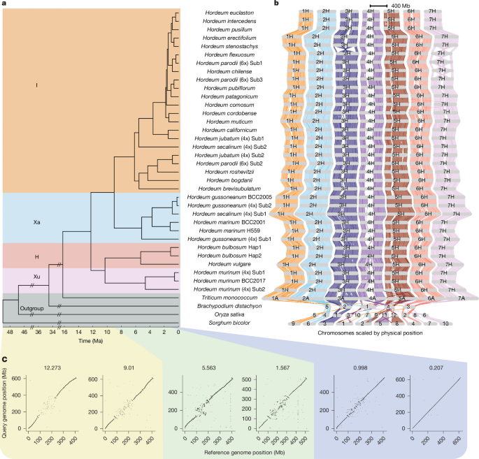
a, Phylogenetic tree of Hordeum species. Sorghum bicolor, Oryza sativa, Brachypodium distachyon and Triticum monococcum were used as outgroups. Divergence times were inferred using 4DTV sites from genome-wide single-copy genes after excluding genomic regions with strong phylogenetic discordance (nRF > 0.21) identified in Extended Data Fig. 6c. Coloured rectangles represent different genome groups. Hap1 and Hap2 represent phased haplotypes of heterozygous diploid H. bulbosum, and Sub1, Sub2 and Sub3 indicate distinct ancestral subgenomes in polyploid species. The background colours represent the genome groups of the species in the following order from top to bottom: I, Xa, H, Xu and outgroup species. b, GENESPACE synteny plot among 34 Hordeum haplomes and four outgroup genomes. Grey bars represent chromosomes arranged by genomic position. For visualization purposes, the chromosomes of the smaller outgroup genomes (S. bicolor, O. sativa and B. distachyon) were proportionally enlarged by a factor of five. c, Dot plot comparisons of chromosome 4H across genomes diverged at different times. Two species were randomly selected from each phylogenetic node for sequence alignment (Supplementary Table 11). Six representative comparisons are shown, with the remaining comparisons presented in Extended Data Fig. 3a. The number displayed at the top of each alignment represents the estimated divergence time between the species shown on the x axis and those shown on the y axis.
Based on the annotated gene sets of all species, we constructed a gene-based Hordeum pangenome. Overall, 42.4% of genes were classified as core genes, 56.5% as shell genes and 1.1% as cloud genes (Extended Data Fig. 1b,c). Gene ontology enrichment analysis showed that phosphorylation- and kinase-related functions were enriched among core genes, ATP and RNA binding were enriched among shell genes, and defence response and oxidative stress response were enriched among cloud genes (Supplementary Fig. 29). Nucleotide-binding leucine-rich repeat (NLR) genes are key components of the plant immune system and have essential roles in resistance to fungal and other pathogens32,33. A map of their diversity is critical for advancing our understanding of disease resistance mechanisms in crops. Analysis of NLR genes revealed that I genome species contain significantly more NLR genes than the other Hordeum genome groups (Welch’s t-test, P = 1.8 × 10⁻⁶) (Extended Data Fig. 2a,b). To further characterize this diversity, we constructed an NLR pangenome across Hordeum haploid genome equivalents (haplomes), comprising 800 orthogroups, of which 13.75% were classified as core, 27.75% as shell and 58.50% as cloud gene families (Extended Data Fig. 2c). In addition, NLR gene clusters were significantly less abundant on chromosomes 4H and 5H than on the remaining chromosomes (Wilcoxon test, P < 2.2 × 10⁻¹⁶) (Extended Data Fig. 2d). Similarly, genome-wide analyses of pentatricopeptide repeat (PPR) proteins and mitochondrial transcription termination factors (mTERFs) revealed significant expansions of restorer-of-fertility-like (RFL) subgroups in the I and Xa genome groups relative to the H and Xu genome groups. Because RFL proteins are involved in fertility restoration in plants carrying cytoplasmic male sterility (CMS)34, these expansions suggest that the smaller RFL repertoires of the H and Xu genome groups are derived rather than ancestral (Supplementary Fig. 30a–e and Supplementary Table 9). Expansion of RFL-PPRs was most pronounced in the I genome group, whereas RFL-mTERFs were significantly expanded in both the I and Xa genome groups. Notably, RFL-mTERF genes clustered on the short arm of chromosome 6H exhibited extensive copy-number variation between Xa–I and H–Xu genome groups (t-test, P = 5.2 × 10⁻⁶) (Supplementary Fig. 30f). This region includes the Rfm3 locus, which partially restores fertility in plants carrying the msm1 cytoplasm used in hybrid barley breeding35 (Supplementary Fig. 30g).
To assess the feasibility of graph-based pangenome analyses across highly diverged Hordeum genomes, we constructed a pangenome graph using Progressive Cactus and hal2vg, comprising 2.53 billion nodes and 3.46 billion edges (68.7 Gb). Approximately 68% of nodes represented single-base variants, illustrating the extensive sequence divergence captured by the graph. Although computationally intensive tasks such as indexing remained infeasible (Methods), we successfully performed global analyses of core, shell and cloud sequence content, graph saturation, sequence conservation and variant diversity (Supplementary Figs. 31–34). These results demonstrate both the potential of graph-based approaches for genus-wide comparative genomics and the need for more scalable methods for graph exploration and interpretation.
Large structural variations reshape proximal region
Previous studies have inferred the evolutionary relationships among Hordeum species from plastome and partial gene sequences1,17. However, the relationships among some species remained weakly supported. In this study, we reconstructed a maximum-likelihood tree using a genome-wide single-copy gene set. Unlike previous phylogenies1,17, our species tree resolved all major evolutionary relationships with maximum bootstrap support, particularly among the recently diverged I-genome species (Supplementary Fig. 35). To further evaluate the robustness of these relationships, we reconstructed an independent coalescent-based species tree using ASTRAL-Pro3 (Supplementary Fig. 36), which integrates individual maximum-likelihood gene trees, and a genome-wide phylogeny inferred by CASTER from whole-genome multiple sequence alignments (MSAs) (Supplementary Figs. 37 and 38). We also estimated the divergence times of these species using fourfold degenerate third-codon transversion (4DTV) sites, excluding genomic regions identified as putatively derived from ancient hybridization (Supplementary Table 13). We estimated the divergence time between H and Xu at 10.3 million years ago (Ma), whereas I and Xa diverged around 9 Ma. The crown-group age of Hordeum dates back approximately 12.27 Ma (Fig. 1a and Supplementary Table 10). The chromosomes of Triticeae species exhibit high collinearity at their distal chromosome regions36, which is also the case in Hordeum (Fig. 1b). However, when aligned, the proximal regions show substantial loss of collinearity and highly fragmented alignments. Whole-genome comparisons across Hordeum species revealed that chromosomal rearrangements accumulated progressively with evolutionary divergence, contributing to the loss of collinearity and increasingly fragmented alignments in proximal chromosomal regions (Fig.1c, Extended Data Fig. 3a, Supplementary Figs. 39–44 and Supplementary Table 11). Quantification of reverse-orientation alignments across all Hordeum haplomes further demonstrated that putative inversions accumulated significantly more rapidly in proximal than in distal chromosome regions during Hordeum evolution (Supplementary Fig. 45). Among the seven chromosomes, chromosome 4H exhibited the most extensive loss of proximal collinearity (Supplementary Table 12). Recently diverged species retained strong chromosome-scale collinearity despite the presence of numerous structural variants, whereas comparisons between the deeply diverged H–Xu and Xa–I genome groups (more than 9 Ma) showed almost complete fragmentation of proximal collinearity (Fig. 1c, Extended Data Fig. 3a and Supplementary Figs. 39–44). To estimate the size of non-collinear regions, we applied normalized coverage to identify these regions in species that diverged more than 9 Ma (Extended Data Fig. 3c,d, Supplementary Figs. 46–50 and Methods). In total, we determined the genome-wide distribution of non-collinear regions across chromosomes in Hordeum, with a cumulative size of 855 Mb identified in the H. vulgare genome (Supplementary Table 12). Given the central role of TEs in genome evolution, we compared TE composition between proximal and distal chromosome regions. Proximal regions contained a significantly higher proportion of TEs than distal regions (one-sided paired Wilcoxon test, P = 9.31 × 10⁻¹⁰), primarily due to an increased abundance of LTR/Gypsy retrotransposons (one-sided paired Wilcoxon test, P = 9.31 × 10⁻¹⁰) (Extended Data Fig. 4a,b and Supplementary Fig. 51). Together with the accumulation of large chromosomal rearrangements, these observations motivated a ‘stretch and twist’ model describing two complementary processes underlying the progressive loss of collinearity. The stretch component represents alignment displacement caused by TE amplification, whereas the twist component represents large-scale chromosomal rearrangements driven by structural variation (Extended Data Fig. 4c).
Large structural variations reveal hybridization
In contrast to the dynamic structural variations found in proximal regions, the distal regions displayed more conserved, shared structural variations. This highlights that the extensive loss of collinearity in proximal regions precludes reliable identification of structural variants across more distantly related Hordeum species. Notably, large structural variations in the distal regions were predominantly inversions. On chromosomes 3H and 7H, we identified two large inversions spanning nearly the entire chromosome and present in multiple species (Extended Data Fig. 4d). In total, 1,407 inversions larger than 2 Mb were identified across Hordeum species (Extended Data Fig. 4d). The construction of a comprehensive inversion map revealed six inversions on chromosome 1H that were unexpectedly shared across divergent phylogenetic lineages (Fig. 2a and Extended Data Fig. 5). We hypothesized that these large-scale structural variations might have originated from introgression events involving extensive chromosomal segments. We constructed a phylogenetic tree using the single-copy gene set from these regions to test this hypothesis. The resulting tree, resolved with maximum bootstrap support, confirmed that these structural variations are shared between one clade of the I genome group and the H–Xu genome groups (Fig. 2b). Moreover, 10 extant diploid Hordeum species diversified within 1.68 million years following the inferred hybridization event, whereas no comparable radiation occurred in other phylogenetic lineages during the same period (Figs. 1a and 2b and Extended Data Fig. 5). Notably, the alternative phylogenetic topology extends across contiguous chromosomal regions of approximately 200 Mb rather than isolated loci, indicating the inheritance of chromosome-scale haplotypes that are more consistent with ancient introgression than with stochastic gene tree discordance or incomplete lineage sorting.
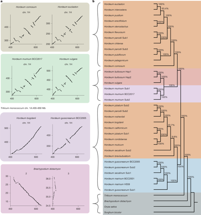
a, Dot plot comparisons of the chr. 1A:400–650 Mb region between T. monococcum and seven representative genomes selected for clarity. The remaining genome comparisons are shown in Extended Data Fig. 5. Colours indicate different clusters and are consistent between this panel and Extended Data Fig. 5. b, Phylogenetic tree based on single-copy genes within the chr. 1A:400–650 Mb region of T. monococcum. Coloured rectangles represent different genome groups. Bootstrap values are shown below each node. Approximately unbiased (AU) test based on concatenated local single-copy genes supports the local tree (p-AU = 1.0) and rejects the reference tree (p-AU = 1.4 × 10−42).
To identify additional signatures of ancient hybridization across the genus, we developed a genome-wide scanning approach based on local phylogenetic discordance among single-copy genes. The single-copy gene set was partitioned into sliding windows, and normalized Robinson–Foulds (nRF) distance was calculated between local phylogenetic trees and the genome-wide species tree (Extended Data Fig. 6a). Peaks in nRF values indicate genomic regions with phylogenetic histories that deviate from the species tree and therefore represent candidate introgression events. Here, we define hybridization footprints as large chromosomal segments shared among multiple descendant species that consistently exhibit an alternative phylogenetic relationship relative to the genome-wide species tree. Using an empirical threshold of 0.21 derived from the genome-wide nRF distribution to distinguish discordance peaks from background variation (Extended Data Fig. 6b and Supplementary Fig. 52), we recovered the chromosome 1H hybridization signal, validating the genome-wide scanning approach. Additionally, we detected more than ten consecutive windows with strong phylogenetic discordance signals at multiple regions (Extended Data Fig. 6c and Supplementary Fig. 52). To further explore the underlying causes of these inconsistencies, we reconstructed local phylogenetic trees using the single-copy gene sets from these regions (Extended Data Fig. 6e,f, Supplementary Figs. 53–58 and Supplementary Table 13). Regions in which local phylogenies consistently supported a specific alternative relationship across a large chromosomal segment were interpreted as evidence of ancient hybridization. By comparing the regions that exhibited phylogenetic discordance with the whole-genome tree, we identified two large-scale segmental exchanges occurring within Hordeum jubatum, with maximum bootstrap support (Extended Data Fig. 6e,f and Supplementary Table 13). Surprisingly, this large-scale segmental exchange explains the major duplication and deletion pattern previously identified on chromosome 5H relative to the H. vulgare reference genome (Supplementary Figs. 12, 56, 59 and 60). The exchanged regions in the two H. jubatum subgenomes are each more closely related to different ancestral genomes, indicating that the apparent duplication and deletion resulted from ancestral segmental exchange rather than independent copy-number changes. (Extended Data Fig. 6d). In the allotetraploid H. gussoneanum, extensive segmental exchanges were detected between the two subgenomes on chromosomes 2, 5 and 7 (Extended Data Fig. 6e, Supplementary Figs. 53, 55 and 57 and Supplementary Table 13). In the allohexaploid H. parodii, subgenome 1 carried a large chromosomal segment on chromosome 7 derived from Hordeum stenostachys, whereas subgenomes 2 and 3 exhibited an additional segmental exchange on chromosome 4 (Extended Data Fig. 6f, Supplementary Figs. 54, 55 and 58 and Supplementary Table 13). Together, these megabase-scale structural variants preserve signatures of ancient interspecific hybridization and large-scale chromosomal exchange that are not evident from genome-wide phylogenies alone, providing new insights into the complex evolutionary history of Hordeum.
Horizontal gene transfer
Genetic variation is essential for species evolution. Beyond sexual reproduction, horizontal gene transfer (HGT) serves as an evolutionary shortcut for acquiring novel genes. Traditionally considered rare in vascular plants, genomic advances have revealed widespread occurrences of HGT, challenging prior assumptions37,38. Our previous research demonstrated extensive HGT in Hordeum. Notably, species within section stenostachys (I genome; 16 out of 22 diploid species) possess ribosomal DNA (rDNA) acquired from grasses in the subfamily Panicoideae (for example, Panicum, Paspalum and Setaria)39,40. The oldest transfers (from Panicum), estimated to have occurred between 5 and 1.7 Ma, resulted in large genomic insertions on chromosome 5H, some spanning over 400 kb and containing TEs and protein-coding genes41. Here, we identified Panicoideae-derived nuclear genes across 20 diploid Hordeum species, with H. vulgare serving as a negative control39,41. Our analysis revealed 611 foreign genes that corresponded to 126 orthogroups, predominantly matching Paspalum (63%) and Panicum (22%) (Extended Data Fig. 7a and Supplementary Tables 14 and 15). The extent of HGT varied, with Hordeum flexuosum carrying the highest number of foreign genes (68 genes corresponding to 43 orthogroups) (Extended Data Fig. 7a). These findings align with studies indicating that grasses frequently exchange genetic material42,43. HGT frequency correlates with Hordeum phylogeny, with Mediterranean and West Asian species exhibiting fewer transferred genes than their South American counterparts. This supports the hypothesis that HGT has a cumulative impact on eukaryotic evolution44. The presence of a single panicoid gene in H. bulbosum and H. murinum can be explained by the introgression of chromosomal segment 1H from I genome species, rather than by an early HGT event predating the diversification of Hordeum (Fig. 2b and Extended Data Fig. 6c). Chromosomal mapping indicates that horizontally transferred genes are distributed across all seven Hordeum chromosomes, with chromosome 5H carrying the largest number (Extended Data Fig. 7b). These genes are significantly enriched in the distal regions of chromosome arms. Although distal regions generally contain higher local gene densities, negative binomial regression analysis showed that gene density explains only a small fraction of the observed variation in HGT abundance (pseudo-R2 = 0.034; Supplementary Fig. 61), indicating that higher gene density alone cannot account for the distal enrichment of HGT genes. Although co-transfer of genes remains uncertain, previous research suggests that large fragments of foreign DNA may be transferred together41,43. A substantial fraction (82 out of 126) of Panicoideae-derived orthogroups lack native Hordeum homologues, indicating novel gene acquisition. Functional annotation suggests that these genes may have roles in key physiological processes such as auxin transport, light response and transcription regulation. RNA sequencing (RNA-seq) analysis detected at least one expressed HGT gene in 73 out of 126 orthogroups (Extended Data Fig. 7c and Supplementary Table 16). The potential adaptive significance of these genes warrants further investigation. Our genus-wide analysis establishes Hordeum as a model system for studying the evolutionary impact of HGT.
TE evolution in Hordeum
The genome assembly sizes of Hordeum species range from 2.90 Gb to 10.9 Gb and are highly correlated with previous flow-cytometric estimates45 (Fig. 3a). After accounting for the direct effects of polyploidization, the haplomes exhibit pseudomolecule sizes ranging from 2.85 Gb to 4.68 Gb. Apart from a 19 Mb duplication detected in the subgenome of H. jubatum, no large duplication events were identified (Supplementary Figs. 59–60). A strong correlation was observed between total TE content and haplome size (Fig. 3b), confirming that TE accumulation has significantly contributed to genome size variation in Hordeum. LTR retrotransposons were identified as the primary drivers of these changes, although DNA transposons also had a role (Fig. 3c). Correlation analyses of individual transposon superfamilies showed that multiple TE families contributed to genome size variation, although overall TE abundance remained the strongest predictor of haplome size (Supplementary Fig. 62a). We selected transposons annotated in the TREP database with an average content above 20 Mb and examined their variation across different Hordeum haplomes. These TE families clearly differentiated the major evolutionary lineages of Hordeum (Supplementary Fig. 62b). To investigate lineage-specific TE dynamics in greater detail, we focused on three LTR retrotransposon families (BARE1, Sabrina and BAGY2) and used TEpop46 to reconstruct their diversification histories. TE subfamilies correspond closely to the major Hordeum clades (Fig. 3d and Extended Data Fig. 8a,b), demonstrating lineage-specific amplification histories that contributed to genome size evolution.
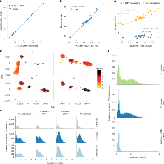
a, Collinearity between assembly size and DNA content (n = 25, two-sided linear regression, P < 2.2 × 10⁻¹⁶). b, Collinearity between pseudomolecule size and TE content (n = 34, two-sided linear regression, P < 2.2 × 10⁻¹⁶). c, Correlation between pseudomolecule size and retrotransposon (n = 34, two-sided linear regression, P = 1.24 × 10⁻¹⁴) and DNA transposon content (n = 34, two-sided linear regression, P = 0.134). d, Principal component analysis (PCA) of 68,707 full-length RLG_BAGY2 retrotransposon sequences across Hordeum species. Each dot represents one retrotransposon; colours indicate estimated insertion times (Ma). e, Distribution of insertion times of full-length LTR elements in H. jubatum, H. californicum and Hordeum roshevitzii. H. californicum and H. roshevitzii are the respective diploid progenitors of subgenomes 1 and 2 in H. jubatum1. f, Inference of post-allopolyploidization TE insertion dynamics in tetraploid H. murinum subsp. murinum (BCC 2009) based on full-length LTR/Copia elements shared between subgenomes. Subgenome-derived TEs represent TE insertions detected in one subgenome that are shared with the other subgenome but absent from the corresponding diploid progenitor, reflecting TE accumulation after subgenome fusion. The onset of the insertion peak indicates the estimated timing of allopolyploid formation. H. murinum subsp. glaucum (BCC 2017) is the diploid progenitor of subgenome 1 in BCC 2009 (ref. 1).
To investigate TE evolution following polyploidization, we compared the TE landscapes of three independently formed tetraploid genomes with those of their diploid progenitors. The three polyploid species exhibited distinct evolutionary trajectories. In H. murinum, TE expansion was minimal (Extended Data Fig. 8c and Supplementary Table 17). In H. jubatum, both subgenomes were smaller than their diploid progenitors (Fig. 3e and Supplementary Table 17). By contrast, Hordeum secalinum experienced extensive TE proliferation, resulting in substantial genome expansion (Extended Data Fig. 8d and Supplementary Table 17). Notably, LTR/Gypsy elements showed the greatest expansion relative to the diploid progenitors and therefore contributed most to genome expansion in H. secalinum (Supplementary Table 17). Additionally, the Vagabond TE family showed renewed activity following tetraploidization, with significantly higher activity in the tetraploid genome than in either its diploid progenitors or the alternative subgenome (Extended Data Fig. 8e and Supplementary Figs. 63 and 64). To avoid bias introduced by large segmental exchanges between subgenomes, we excluded genomic regions inferred to originate from ancient hybridization before estimating TE insertion ages (Supplementary Table 13 and Supplementary Fig. 65). Although subgenome differentiation alone does not permit precise dating of tetraploid formation, post-polyploid TE dynamics can be reconstructed from TE insertions. Specifically, we inferred the timing of subgenome fusion from the insertion ages of full-length TEs shared exclusively between subgenomes but absent from their respective diploid progenitors (Fig. 3f, Extended Data Fig. 8f,g and Supplementary Figs. 65 and 66). These shared insertions must have occurred after polyploid formation, thereby providing temporal information on the origin of the polyploid genomes and subsequent TE activity. Our findings underscore that TE content is the primary determinant of genome size variation in Hordeum. Tetraploidization does not always lead to genome expansion relative to diploid ancestors; we also observed genome contraction. Nevertheless, post-polyploid LTR insertions provided an independent estimate of the timing of polyploid formation and new insights into the evolutionary history of tetraploid and hexaploid Hordeum genomes.
Sequence conservation across species
Whole-genome MSAs provide a framework for investigating sequence conservation and divergence across species. We therefore generated a whole-genome MSA of Hordeum haplomes using Progressive Cactus47. In total, we identified 170.4 Mb of shared aligned sequences across the Hordeum genomes (Extended Data Fig. 9a). As expected, rapidly evolving pericentromeric regions showed fewer alignments, whereas chromosome distal ends exhibited higher alignment densities (Extended Data Fig. 9b). The rapid contraction of these alignments is probably due to substantial reshaping of Hordeum genomes by TE activity over the past 12 million years. To further investigate sequence conservation across different functional genomic regions, we analysed open chromatin regions identified by assay for transposase-accessible chromatin with sequencing (ATAC–seq) together with annotated genomic features in eight Hordeum haplomes (Supplementary Table 18). Untranslated region sequences were the most highly conserved non-coding regions and were lost at a slower rate before the divergence of barley and wheat. By contrast, open chromatin regions exhibited a loss pattern similar to introns, whereas promoter regions underwent more rapid turnover (Extended Data Fig. 10a). Additionally, we used phastCons to identify 74.7 Mb of conserved elements across Hordeum genomes (Extended Data Fig. 10b,c). Among all conserved bases, 69.0% overlapped annotated genes and 6.0% overlapped open chromatin regions. Conversely, 44.7% of annotated gene bases and 31.9% of open chromatin bases overlapped conserved elements. Conserved elements were significantly enriched in both annotated genes (odds ratio = 138.0) and open chromatin regions (odds ratio = 27.4), with substantially stronger enrichment in genes, indicating stronger evolutionary constraint on coding sequences than on regulatory regions (Extended Data Fig. 10c).
Overall, our findings indicate that regulatory elements undergo substantially faster evolutionary turnover than coding sequences, generating extensive regulatory variation that may provide a valuable source of alleles for barley improvement. By contrast, the high conservation of coding genes provides opportunities for comparative functional analyses and cross-species transfer of biological knowledge.
Natural variation in vernalization
In cultivated barley, spring and winter growth habits are largely determined by the vernalization genes VERNALIZATION 1 (VRN1), a MADS-box transcription factor, and VERNALIZATION 2 (VRN2), which is encoded by a cluster of zinc-finger/CCT (ZCCT) genes. In winter barley, prolonged cold induces VRN1 expression, which represses VRN2 and thereby permits flowering48,49. Flowering of winter varieties requires repression of VRN2 by cold-induced VRN1 (ref. 49). By contrast, spring barleys often carry deletions in the first intron of VRN1 and lack VRN2, eliminating their vernalization requirement50,51,52. Intermediate facultative types combine the vernalization-sensitive VRN1 with a non-functional VRN2 locus. It remains largely unexplored how wild Hordeum species regulate flowering across diverse climates.
Examining VRN1 in Hordeum genomes revealed extensive variation in the promoter and the regulatory first intron (5.7 kb to 19.5 kb) caused by TEs (Supplementary Table 19). To assess the functional effect of this variation, we recorded flowering time of 14 wild Hordeum species and 4 barley controls under non-vernalizing conditions with a 14 h light:10 h dark photoperiod (Fig. 4a and Extended Data Fig. 11a). Notably, Hordeum cordobense and Hordeum muticum flowered rapidly (approximately 61 days), surpassing spring barley cultivars (Fig. 4a). Both species share a unique 79-bp deletion in VRN1 intron 1 critical region51, suggesting a role in reducing the vernalization requirement (Extended Data Fig. 11b). All species contained the VRN2 locus with one to seven ZCCT copies (Supplementary Table 19). A key finding was an inverted repeat of two ZCCT genes in H. cordobense, Hordeum californicum, H. muticum and H. jubatum (Supplementary Fig. 67). Because inverted repeats may trigger RNA interference (RNAi)53, we expected silencing of VRN2 and a spring-type phenotype. Surprisingly, only H. cordobense and H. muticum flowered early (Fig. 4a,c and Extended Data Fig. 11a). Detailed analysis of H. cordobense revealed a non-functional ZCCT-1 owing to a premature stop codon, and the absence of a polyadenylation signal in the ZCCT-2/ZCCT-3 inverted repeat linker, enabling read-through transcription (detected as an aberrant mRNA transcript), hairpin RNA formation and small RNA production (Fig. 4b,d, Extended Data Fig. 11c and Supplementary Fig. 68). Winter-type H. californicum carried additional functional ZCCT copies and a polyadenylation signal in the inverted repeat linker that probably prevented RNAi, thus maintaining the VRN2 repressive function (Fig. 4b,e). This aligns with the expression of VRN1, VRN2 and their target FLOWERING LOCUS T1 (FT1) in the analysed species (Fig. 4f). These findings highlight that genetic diversity shapes vernalization in Hordeum. The studied spring-like accessions carry the 79-bp VRN1 deletion alongside disrupted or silenced VRN2, whereas winter-like genotypes retain functional ZCCT copies. Together, our results indicate that adaptation to spring growth habit in wild Hordeum species has targeted the same genes and variant types as in cultivated barley, pointing to conserved mechanisms of flowering-time adaptation.
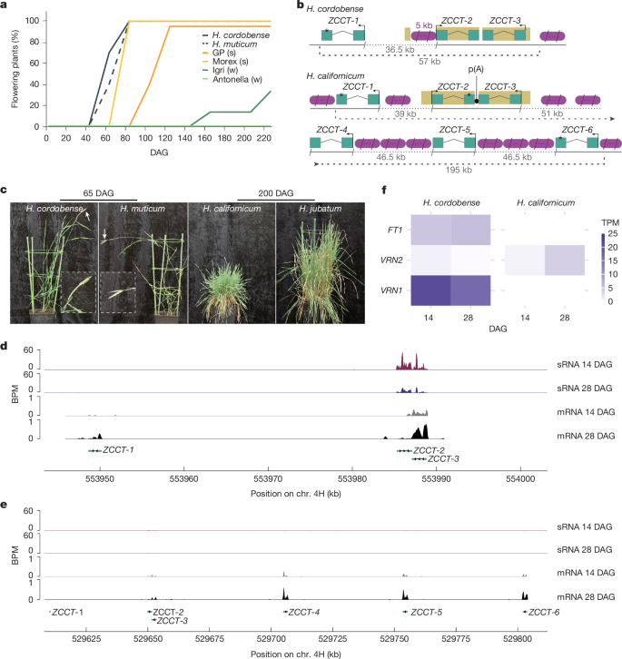
a, Percentage of H. cordobense and H. muticum plants (n = 10 per species) that flower under non-vernalizing conditions. The cultivars Golden Promise (GP) and Morex serve as spring-type (s) controls and cultivars Igri and Antonella serve as winter-type (w) controls. DAG, days after germination. b, Structure of the VRN2 locus in H. cordobense with three ZCCT genes, and in H. californicum with six ZCCT genes. The scheme is not to scale. Teal rectangles represent exons, asterisks indicate stop codons, purple ovals are TEs, the black dots indicate a polyadenylation (p(A)) signal and sand-coloured regions are inverted repeats. c, Phenotypes of four Hordeum species with contrasting VRN2 locus structures at 65 and 200 DAG. Arrows mark visible spikes. d,e, Mean distribution of RNA-seq and small RNA (sRNA)-sequencing reads over three biological replicates normalized to bins per million (BPM) mapped reads in H. cordobense (d) and H. californicum (e) across the VRN2 locus at 14 and 28 DAG. Read mapping at the H. cordobense ZCCT-3 locus suggests the presence of improperly spliced, probably aberrant transcripts. f, Transcripts per million (TPM) values at 14 and 28 DAG in H. cordobense and H. californicum.
Conserved control of glume development
The glume is a distinctive floral organ in the grass family, which lacks a direct counterpart in dicotyledonous plants54. It appears as one or multiple pairs of bract-like structures subtending single or multiple fertile florets. Glume size and shape vary widely, from large lemma-like structures in Triticum species to rudimentary axillary buds in Oryza. In wild grasses, glume morphology influences seed dispersal, reproductive success and defence against biotic stress55. In cultivated cereals, domestication has favoured reduced glume size and roughness, facilitating easier threshing. In Hordeum, each floret possesses a pair of glumes positioned on the periaxial side, with considerable variation in length, width and awn extension across species (Fig. 5a). Transcriptomic profiling of five diploid species carrying the I genome (H. erectifolium, Hordeum pusillum, Hordeum intercedens H. stenostachys and Hordeum euclaston) identified spike-specific genes expressed in young spikes at early (Waddington stages 3–6 (W3–6)) and late (W9–10) developmental stages56 (Supplementary Table 21). Genes were classified as spike-specific if their transcript abundance in the remaining 11 out of 13 analysed tissues was less than 5% of their combined expression in the 2 spike samples. Five genes were consistently expressed across species, suggesting conserved regulatory mechanisms (Extended Data Fig. 12a and Supplementary Table 21). These genes encode a C2H2-type zinc-finger transcription factor, an auxin response factor, a TCP transcription factor, a subtilisin protease (SBT) and a MADS-box transcription factor. Three were predominantly expressed during early spike development, one at later stages and one at both stages (Extended Data Fig. 12b). In rice, loss-of-function mutations in NONSTOP GLUMES1 (NSG1), the orthologue of the C2H2-type zinc-finger transcription factor, result in uncontrolled glume growth57. Amino acid variations in this gene across Hordeum species along with glume variations suggested a relevance in regulating glume development (Fig. 5a and Supplementary Fig. 69). Mutations in its cultivated barley orthologue (EOG1) lead to the elongated outer glume (eog1) phenotype (Fig. 5b). These mutants develop enlarged glumes on the central fertile spikelet, with glume awns extending to lemma-awn length, giving the spike a brushy appearance (Extended Data Fig. 12c,d). Scanning electron microscopy (SEM) revealed developmental divergence between wild-type and eog1 mutants as early as W3.5 (Fig. 5c). By integrating comparative genomics across Hordeum with tissue-specific expression data and cultivated barley mutant resources, we identify EOG1 as a conserved regulator of glume development.
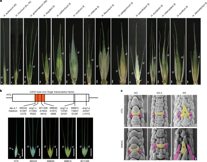
a, Central spikelet from representative Hordeum species exhibiting glume morphology diversity. gl, glume. Scale bars, 500 μm. b, Allelic variations of a C2H2-type zinc-finger transcription factor gene (HORVU.MOREX.r3.2HG0170820.1) in cultivated barley (H. vulgare) lead to glume elongation. The rectangle denotes the exon or full-length coding sequence, with the red rectangle indicating the C2H2-type zinc-finger domain. The asterisk marks a premature stop codon. HTX (Hatiexie) represents the wild type, which exhibits suppressed glume development, whereas the mutants exhibit elongation in glume growth. The mutant allele lep-e.1 (ref. 59) carries a deletion allele of the EOG1 gene. Scale bars, 1 cm. c, Differentiation on the spikelet morphogenesis along Waddington stage between the wild-type HTX and the induced mutant M9630. W3, glume primordial present; W3.5, floret primordial present; W5, carpel extending. le, lemma. Scale bars, 100 μm.
Discussion
The chromosome-scale genome assemblies presented here provide a foundation for investigating the evolutionary history of the genus Hordeum. Chromosome-scale resolution enables us to investigate how structural variations have shaped genome evolution, particularly in disrupting chromosomal collinearity. Traditionally, grass genomes were thought to possess relatively stable chromosome structures58; however, our findings challenge this assumption. Extensive structural variations and chromosomal rearrangements have contributed substantially to genomic divergence, ultimately resulting in the near-complete loss of collinearity in proximal regions. These rearrangements not only mark evolutionary divergence but also provide insights into the processes underlying speciation within Hordeum. Structural variations accumulated at markedly different rates across chromosome regions. Whereas proximal regions exhibit high variability, distal regions evolve more slowly. This uneven evolutionary rate has preserved footprints of ancient hybridization events across the genus, offering a historical record of interspecific gene flow. These findings provide empirical evidence for ancient hybridization and genome fusion during Hordeum evolution and establish a framework for identifying compatible genomic segments in future interspecific breeding efforts.
Nevertheless, whether the large inversions identified in this study contribute to adaptive evolution, reproductive isolation or other phenotypic consequences remains unknown and warrants future functional investigation. Whole-genome MSAs enabled us to compare genome-wide conservation across Hordeum species. Compared with animal genomes, which often display strong interspecies conservation, plant genomes—especially within rapidly evolving genera such as Hordeum—undergo dynamic changes driven by short generation times and rapid transposon expansion. These processes fuel the ongoing remodelling of plant genomes, resulting in high variability even among closely related taxa. Despite this rapid evolution, many genes remain conserved, whereas regulatory elements exhibit considerable turnover. This contrast offers unique opportunities: lineage-specific regulatory innovation can be harnessed for crop improvement, while core gene functions are retained. For example, regulatory elements associated with vernalization responses were found to vary across Hordeum species, suggesting that novel regulatory variants could be introduced into cultivated barley to fine-tune flowering behaviour. Beyond expanding genomic resources for Hordeum, this work provides a framework for investigating structural genome evolution, reconstructing complex evolutionary histories and harnessing genetic and regulatory diversity for barley improvement.
Methods
Plant material
Plant material was obtained from genebanks at Institut für Pflanzgenetik und Kulturpflanzenforschung (IPK) Gatersleben, the US Department of Agriculture and the Nordic Genetic Resource Center. Accession numbers are listed in Supplementary Table 1.
HMW DNA extraction and HiFi sequencing
Plants were grown under greenhouse conditions and high molecular weight (HMW) DNA was isolated from young leaf tissue according to published protocols10,60. Construction of HiFi libraries and Circular Consensus Sequencing using the PacBio Sequel IIe instrument (Pacific Biosciences) were essentially as described previously19. HiFi sequencing was done at IPK Gatersleben, Genomics and Transcriptomics Laboratory, Heinrich Heine University, Berry Genomics Co., Novogene and the University of Wisconsin Biotechnology Center DNA Sequencing Facility.
Hi-C sequencing
In situ Hi-C libraries were prepared from young seedlings according to the previously published protocol, using DpnII for the digestion of crosslinked chromatin. Libraries were prepared as described61. Samples were quantified62 and sequenced with standard protocols from Illumina using Illumina NovaSeq 6000 devices (Illumina) at IPK Gatersleben and Novogene.
Optical genome mapping and hybrid scaffolding
A clone of the same H. erectifolium individual plant that was sequenced using PacBio HiFi was used for the construction of the optical genome map (OGM). A total of 2.5 million nuclei, purified from young leaves by flow cytometry, were embedded in agarose miniplugs and treated with proteinase K, following the protocol of Šimková et al.63. A total of 525 ng of HMW DNA was directly labelled at DLE-1 recognition sites using the standard Bionano Prep Direct Label and Stain protocol (Bionano) and analysed on the Bionano Saphyr platform. The resulting dataset, comprising 1.5 Tb of single-molecule data with an N50 of 247 kb, provided approximately 341× coverage of the H. erectifolium genome. This dataset was used to generate a de novo OGM assembly using Bionano Solve software (v3.6.1_11162020) with the standard configuration file optArguments_nonhaplotype_noES_noCut_DLE1_saphyr.xml.
To improve the contiguity of the PacBio HiFi assembly, the automatic hybrid scaffold pipeline integrated in Bionano Solve was run using the OGM assembly. The default DLE-1 Hybrid Scaffold configuration file was applied with the ‘resolve conflict’ option for conflict resolution. Conflicts between the sequence assembly and the OGM were manually curated and the pipeline was subsequently re-run using a modified conflict_cut_status.txt file.
Transcriptome sequencing
Plants were grown under greenhouse conditions and total RNA was isolated from different tissues and developmental stages (Supplementary Table 5) using the RNAeasy Plant Mini Kit (Qiagen, Hilden, Germany) or with Trizol reagent (Invitrogen) according to the manufacturers’ protocols. RNA-seq was performed on replicated bulk sample representing a specific developmental stage or tissue type. RNA-seq of individual samples and PacBio IsoSeq of RNA pools was performed as described previously10. Library construction and sequencing on Illumina NovaSeq 6000 devices (Illumina RNA-seq) and PacBio Sequel IIe (instruments) was done at IPK Gatersleben, Biomarker Technologies (BMK), the Genomics and Transcriptomics Laboratory at Heinrich Heine University Düsseldorf, Kazusa DNA Research Institute or Berry Genomics. The PacBio IsoSeq sequencing data was processed with the isoseq3 (v3.8.2) pipeline (PacBio - IsoSeq3, 2018/2024). The ploy-A tails were trimmed and concatenated transcripts removed with refine -require-polya-min-polya-length 12 teloprime.fasta. To generate non-redundant transcripts, we mapped the full-length non-concatenated reads were mapped to the genome with pbmm2 (v1.10.0) align -preset ISOSEQ -sort -bam-index CSI and redundant transcripts collapsed with isoseq3 collapse -do-not-collapse-extra-5exons.
Genome assembly
PacBio HiFi reads were assembled using hifiasm (v0.13-r308 or v0.15.5-r350 or v0.16.1-r375)64. Pseudomolecules were constructed with the TRITEX pipeline26,27, and chimeric contigs or orientation errors were corrected based on manual inspection of Hi-C contact matrices. For allotetraploid species, subgenomes were phased using a previously developed haplotype-resolved genome assembly strategy10. The origin of the subgenomes and their potential ancestral contributors were previously investigated in detail by Brassac et al.1 To classify subgenomes in the polyploid genome, Mash (v2.3)65 was used to calculate pairwise chromosomal similarities between polyploid chromosomes and candidate ancestral genomes. The resulting distance matrix was used to infer subgenome origin and relationships. In species with high heterozygosity or outcrossing (H. brevisubulatum and H. murinum BBC2017), Hi-C data were incorporated during hifiasm (v0.15.5-r350)64 assembly to collapse haplotypes and assemble a representative haploid genome. Except for H. erectifolium, whose primary contigs were first hybrid-scaffolded using a Bionano optical map, followed by pseudomolecule construction with Hi-C data and the TRITEX pipeline30. Chloroplast genomes were assembled following previously published protocols10. HiFi reads were aligned to the barley cv. Morex chloroplast genome (GenBank accession EF115541) using minimap2 (v2.24-r1122)66 with the parameters -ax map-hifi–secondary=no–sam-hit-only. Alignments with mapping quality <30 were discarded. Aligned reads were converted to FASTQ format using SAMtools (v1.16.1)67 and assembled with Canu (v2.1.1)68 in PacBio HiFi mode with genome sizes from 120 to 400 kb in 10-kb increments. Circular sequences were identified and trimmed using BEDTools (v2.30.0)69 and annotated with GeSeq70. Fully annotated assemblies were aligned to the Morex chloroplast genome using MUMmer4 (v4.0.0beta2)71, and start positions and orientations of the SSC region were adjusted to match the reference using seqkit (v0.9.1)72. k-mer frequencies were calculated using Jellyfish(v2.2.6)73 and analysed with findGSE(v1.94)74 to estimate genome characteristics. Assembly quality, including QV and k-mer completeness, was evaluated using Merqury(v1.3)75.
De novo gene annotation of the Hordeum pangenome
We performed de novo structural gene prediction, confidence classification and functional annotation, following the protocol described in Mascher et al.28. As evidences we used RNA-seq and IsoSeq data as described under above and Poales-filtered protein sequences downloaded from UniProt76 (July 2023). An additional consolidation step was carried out using the liftoff77 tool. In brief, all predicted gene models from one species were lifted over to all other genomes. Using Mikado78, we selected the best mapped gene models and unified all gene predictions accordingly. We classified predicted proteins into high and low-confidence categories. High-confidence proteins had over 80% coverage and were complete, either with significant hits in UniMag or UniPoa but not PTREP (https://trep-db.uzh.ch). Low-confidence proteins were incomplete with hits in UniMag or UniPoa but not PTREP, or were complete without hits in any database.
We benchmarked the annotations with BUSCO (v5.8.0)79 (dataset: poales_odb12), OMARK (omamer verision 2.1.0/omark v0.3.1)80 and psauron (v1.0.6)81.
Construction of the gene-based Hordeum pangenome
Orthogroups based on the primary protein sequences from 27 annotated Hordeum accessions were calculated using Orthofinder (v2.5.5)82. The scripts for the calculation of core, shell and cloud genes are deposited in the repository at https://github.com/PGSB-HMGU/BPGv2. Core genes contain at least 1 gene model from all 27 compared accessions. Shell genes contain gene models from at least 2 Hordeum accessions and at most 26. Genes clustered with genes only from the same genotype were defined as cloud genes. Annotations of H. vulgare Morex and H. bulbosum were not included during the consolidation step. Therefore, to counteract any potential over- or under-presentation of these two species in any of the core, shell or cloud categories, we aligned all cloud genes for H. vulgare cv. Morex and H. bulbosum back to all other genomes and corrected for any missing genes. Gene Ontology-term enrichments were conducted with goatools (v1.4.4)83. Gene-based collinearity plots were drawn with GENESPACE84.
Pan-genome analysis of nucleotide-binding resistance genes
The RGAugury (v2.2)85 pipeline was used to identify from our annotation and classify nucleotide-binding site (NB-ARC) domain-encoding genes into different subgroups, based on domain and motif structures: TNL contain TIR, NBS and LRR domains; CNL contain CC, NBS and LRR domains; RNL contain RPW8, NBS and LRR domains; RN contain RPW8 and NBS domains only; NL contain NBS and LRR domains but lack TIR, CC and RPW8; TN contain TIR and NBS domains only; CN contain CC and NBS domains only; and NBS-only genes contain only the NBS domain. TIR, NBS, LRR, CC and RPW8 refer to the Toll/Interleukin-1 Receptor-like, Nucleotide-Binding Site, Leucine-Rich Repeat, Coiled-Coil and Resistance to Powdery Mildew 8-like domains, respectively. An NLR gene cluster is defined based on the genomic proximity of NLR genes. Specifically, any two NLR genes located within 500 kb of each other are grouped into the same cluster by bedtools (v2.30.0)69. NLR genes were then grouped into clusters using bedtools (v2.30.0)69 merge with a maximum intergenic distance of 250 kb. Only clusters comprising no fewer than three NLR genes were retained. Pan-NLR analysis was performed based on orthogroups identified using OrthoFinder (v2.5.5)82 across all NLR genes. Core orthogroups are defined as orthogroups that contain at least one gene model from each of the compared Hordeum accessions. Shell orthogroups include gene models from at least two and at most 26Hordeum accessions. Gene models that were not assigned to any orthogroup (singletons) or were grouped only with genes from the same genotype were classified as cloud genes.
Pan-genome analysis of PPR and mTERF genes
Open reading frames longer than 100 codons were searched for the presence of PPR and mTERF motifs using hmmsearch from the HMMER suite (http://hmmer.org) using hidden Markov models as defined in Cheng et al.86. for the PPR family and PF02536 from the Pfam 32.0 database (http://pfam.xfam.org)87 for the mTERF motif. Downstream processing of the hmmsearch results for the PPR proteins followed the pipeline described in Gutmann et al.88. The RfCTD domain recently identified as a unique feature of RFL-PPRs89 was included in the gene annotations. P-class and PLS-class genes with scores below 100 and 240, respectively, were excluded from the annotation as they are unlikely to represent functional PPR genes, as defined previously (IWGSC 2018)90.
Graph-based pangenome construction and analysis
The analyses described here used a number of tools from the toolkits vg (v1.61.0)91, odgi (v0.8.3-26-gbc7742ed)92, bcftools (v1.21)67 and seqkit (v2.9.0)72. All scripts used for graph construction and analysis are available at https://github.com/cropgeeks/panHordeum. Owing to computational limitations, we built an alignment of Hordeum whole genomes with Cactus47. We selected H. marinum BCC 2001 over H. marinum H559 on the basis of its higher assembly quality. Genome haplomes were soft-masked with bedtools69 using their respective repeat annotations. The guide tree required for the Cactus alignment was taken from the Orthofinder93 output generated as part of this study. Apart from setting appropriate resource parameters (that is, threads, memory and disk), we ran Cactus with default parameters. We transformed the resulting whole-genome alignment into a super-pangenome graph using hal2vg (https://github.com/ComparativeGenomicsToolkit/hal2vg), with the –noAncestors flag, and then further processed it with vg convert to get the final pangenome graph in GFA format (https://github.com/GFA-spec/GFA-spec). We computed basic graph statistics using odgi stats with the –summarize option, which included graph size, number of nodes, edges, paths and steps. To characterize the conservation of the different segments of the graph, we classified nodes as core, shell, or cloud. A node was considered ‘core’ if it was traversed by all samples’ paths, ‘cloud’ if it was traversed by a single sample’s path, and ‘shell’ otherwise. The same classification was done at the base level. Both computations were performed using the odgi toolkit (implementation details in class_stats.sh). To evaluate the agreement of haplotype sequences with their representation in the graph, we first extracted the linear sequences of all haplotypes as encoded in the graph using odgi paths with the –fasta option. These sequences were subsequently partitioned by source genome using seqkit grep, creating direct pairwise comparisons between input genomes and their graph-encoded counterparts. For each genome pair, we performed exact sequence matching, confirming whether each input sequence (or its reverse complement) was precisely preserved in the graph-encoded version (implementation details available in script fidelity.py). We computed pangenome graph growth curves based on the full graph using odgi heaps with 100 permutations of the input genomes. Results were plotted using script heaps_fit.R distributed with the odgi toolkit92. Whole-graph analysis turned out to be computationally prohibitive (job runtime limits and/or memory requirements) for several of the required tools from the vg and odgi toolkits, given a graph of this size and complexity. We therefore extracted subgraphs equating to individual chromosome paths for H. vulgare cv. Morex, which we used as the basis for all variant analyses. We used vg chunk for subgraph extraction. Variants were called from the chromosome-level subgraphs directly, using vg deconstruct. This generated VCF output containing the full range of variant sizes. To prepare structural variants from the graph for further analysis we broadly followed the variant decomposition approach used by the Human Pangenome Consortium94. This involved the removal of top-level variants of length >100,000 bp with vcfbub (https://github.com/pangenome/vcfbub), realigning alternate alleles against the reference for each variant using vcfwave (vcflib v1.0.2)95, and finally normalizing the resulting variants with bcftools norm67. We then added variant length information (SVLEN) to the VCF files with a custom script to allow extraction of structural variants based on the length difference between reference and alternate allele (>50 bp) and classified structural variations as deletions or insertions based on the directionality of the difference (insertion: string length REF <string length ALT; deletion: string length REF > string length ALT). The resulting VCF files were converted to BED format with bcftools query. Variant density plots were computed with custom R scripts using ggplot2 (v3.5.1)96. To explore the possibility of using the graph for read mapping and genotyping, we attempted to index the graph using vg gbwt/vg index/vg minimizer. This turned out to be computationally prohibitive in terms of job runtime limits on two separate compute facilities used, and thus we were unable to use the graph for the valuation of read mapping. We conducted graph-based conservation analysis with Pansel97, a tool used for calculation of diversity/conservation metrics directly from pan-genome graphs. The default bin size of 1kbp was used, along with all other parameters on default settings. Results were plotted using ggplot2 (v3.5.1)96.
Whole-genome MSA
Single-copy genes were identified using BUSCO (v5.4.6)79 in B. distachyon (v3.0)98, O. sativa (IRGSP-1.0)99, S. bicolor (NCBIv3)99, T. monococcum100, H. vulgare FT11 (ref. 19) and the 29 Hordeum haplomes collected in this study. Protein sequences of BUSCO single-copy genes present in all 34 haplomes were concatenated and aligned using MAFFT (v7.490)101. Well-aligned regions were filtered using Gblocks (v0.91b)102 with parameters -t=extractedp -b4 = 5 -b5=h. A maximum-likelihood phylogenetic tree was then constructed using RAxML (v8.2.12)103 with the PROTGAMMAWAG substitution model and the rapid bootstrap algorithm with 100 replicates. To facilitate genome-wide alignment, all 34 haplomes were masked using RepeatMasker (v4.1.1; http://www.repeatmasker.org) with a pan-genome TE library generated by panEDTA. The masked genomes and the inferred species tree were then used as input for Cactus (v2.6.5)47 to generate whole-genome MSAs. The loss rate of genomic elements was defined as the size of the reconstructed ancestral sequence at the corresponding genomic position in the multiple genome alignment.
Phylogeny and divergence time estimation
To precisely construct phylogenetic trees and estimate divergence times within the genus Hordeum, we included four additional outgroup genomes: B. distachyon (v3.0)98, O. sativa (IRGSP-1.0)99, S. bicolor (NCBIv3)104 (all downloaded from Ensembl Plants; https://plants.ensembl.org/index.html) and T. monococcum100 (https://wheat.pw.usda.gov/GG3/pangenome). We constructed phylogenetic trees using four approaches. The first two methods were based on whole-genome single-copy genes. Orthologous genes were identified from the genomes of our 34 Hordeum haplomes and four outgroup genomes using OrthoFinder (v2.5.5)82, yielding 2,198 single-copy genes. For the concatenation-based approach, the CDS sequences of these genes were concatenated and aligned with MAFFT (v7.490)101, and well-aligned regions were retained using Gblocks (v0.91b)102 with the parameters -t=extractedp, -b4 = 5, -b5=h; phylogenetic inference was then performed in IQ-TREE (v2.2.2.6)105. For the coalescence-based approach, the CDS sequences of each single-copy gene were aligned separately using MAFFT (v7.490)101, high-quality regions were selected with Gblocks (v0.91b)102 using the same parameters, individual gene trees were reconstructed with IQ-TREE (v2.2.2.6)105, and a species tree was inferred from these gene trees using ASTRAL-Pro3 (CASTLES-Pro, v1.23.3.6)106. The remaining two methods were based on whole-genome MSAs generated with Cactus. In the CASTER-pair (CASTLES-Pro, v1.23.3.6)107 approach, the whole-genome MSA was used to infer a phylogenetic tree rooted with S. bicolor, while in the CASTER-site (CASTLES-Pro, v1.23.3.6)107 approach, the whole-genome MSA was analysed similarly but using site-based inference, also rooted with S. bicolor.
To estimate divergence times, genomic regions showing strong phylogenetic discordance (nRF > 0.21) were first excluded based on the genome-wide discordance analysis. 4DTV sites were extracted from MSAs of single-copy genes. Divergence times between barley and outgroup species were obtained from the TimeTree database (https://timetree.org/)108. Finally, species divergence times within the genus Hordeum were estimated using the MCMCtree program in PAML (v4.4)109.
Identify the boundary of the proximal regions
We excluded multiple haplomes from the same species and retained a final set of 32 Hordeum haplomes for comparative analysis. All haplomes pairs were aligned against each other using minimap2 (v2.24-r1122)66 with the parameters -2 -K 5 G -f 0.005 -x asm10, and the resulting alignments were stored in PAF format for visualization via dot plots. For each reference haplomes, we calculated the alignment coverage in non-overlapping 5 Mb windows, considering only alignments with a mapping quality greater than 20. Coverage values were normalized across the haplomes by the average coverage to produce normalized coverage profiles. In species that diverged more than 9 Ma, a bimodal distribution of normalized coverage was observed, allowing a threshold of 0.5 to distinguish distal and proximal regions (Extended Data Fig. 3b,c). Finally, genome-wide alignment and normalized coverage profiles were used to manually define the size and boundaries of proximal and distal regions across all species. Reverse-orientation alignments were extracted as indicators of putative inversion events. Two metrics were calculated for each pairwise comparison: (1) the number of reverse-orientation alignments per Mb and (2) the proportion of bases covered by reverse-orientation alignments. These metrics were separately calculated for proximal and distal chromosomal regions to compare the rates of inversion accumulation during species divergence. Linear regression models including divergence time, chromosomal region type (proximal or distal) and their interaction term were used to evaluate differences in the accumulation rates of reverse-orientation alignments between regions.
Identification of large inversions
All other Hordeum genomes were aligned to the MorexV3 (ref. 28) reference genome using wfmash (v0.9.1-3; https://github.com/waveygang/wfmash) with the parameters -p 90 -l 0. Inversions were then identified using SyRI (v1.5.5)110 with parameters -F P -f–nosnp. Only inversions larger than 2 Mb and located outside of the proximal regions were retained for further analysis.
Detection of introgressed regions using gene tree discordance
Based on the 2,198 single-copy orthologues identified in the section ‘Phylogeny and divergence time estimation’ and using the genome-wide concatenated single-copy gene tree as a reference, we conducted sliding-window gene tree analyses (Extended Data Fig. 6a). All single-copy genes were grouped into non-overlapping windows of 25 genes with a step size of 2 genes. Within each window, protein sequences were aligned using MAFFT (v7.490)101, and well-aligned regions were retained using Gblocks (v0.91b)102 with the parameters -t=extractedp -b4 = 5 -b5=h. Local window trees were built with FastTree (v2.1.11)111 (default GTR + CAT, 20 rate categories), starting from neighbour-joining trees and optimized with minimum-evolution and nearest-neighbour interchange moves; branch support was calculated using Shimodaira–Hasegawa-like values. Each resulting tree was rooted with S. bicolor as the outgroup using ETE3 (v3.1.2)112, and the nRF distance was calculated against the reference tree using the parameter –min_support_src 90. The nRF metric quantifies topological dissimilarity between trees, with values ranging from 0 (identical topology) to 1 (completely different topologies). Based on the nRF distribution, we identified 0.21 as a threshold to separate background from discordant signal peaks (Extended Data Fig. 6b). To evaluate the robustness of discordant region detection, we repeated the sliding-window analyses using alternative parameter settings (30 genes with step sizes of 1 and 5 genes). The major discordance peaks were consistently recovered across different window sizes and step lengths, indicating that peak detection was not sensitive to parameter selection (Supplementary Fig. 52). Genomic regions containing at least 10 overlap windows with nRF ≥ 0.21 were defined as candidate introgressed regions. For each candidate region, we reconstructed local phylogenetic trees using the same procedure as for the genome-wide tree. The topological comparison of these local trees with the reference tree enabled the inference of introgression origins. The AU test113 implemented in IQ-TREE (v2.2.2.6)105, was used to compare local reference trees and local phylogenetic trees. A P value (p-AU) lower than 0.05 indicated that the tree was significantly rejected.
Identification of HGT candidates
Genomes of 20 diploid Hordeum species were searched for potential HGT genes from grasses of the subfamily Panicoideae. Regions of interest were identified in the genomes using BLAST (v2.12.0+)114 against four potential donor species: Panicum hallii (v3.2), Setaria italica (v2.2), Paspalum vaginatum (v3.1) and Paspalum notatum (GCA_036689595.1) (Supplementary Table 10). BLAST results were filtered to retain hits with a sequence identity of ≥95% and an alignment length of ≥150 bp. The same process was applied to H. vulgare cv. Morex (v3), which served as a negative control. H. vulgare is widely recognized as a species that lacks HGT genes from the Panicoideae subfamily39,41,42. Hits from potential donors that were found in both the Hordeum recipient genomes and H. vulgare were excluded from further analysis. This filtering was conducted using the intersect tool from BEDTools (v2.26.0)69, with an overlap threshold of 20%. Finally, the identified regions were compared with newly available annotations, and corresponding candidate genes were extracted. In this step, we identified 5,169 candidate genes.
Phylogenetic validation of HGT candidates
To verify the foreign (that is, Panicoideae) origin of the candidate HGT genes identified as described above, phylogenetic trees were constructed for each candidate. Homologues were retrieved from a set of representative Poaceae species and two outgroups (Ananas comosus and Musa acuminata) (Supplementary Table 10) using BLASTn (e-value cutoff of 10−10). The retrieved sequences were aligned with the Hordeum HGT gene candidates using MUSCLE (v3.8)115. The alignments were trimmed using trimAl (v1.2) with an automated trimming method116. Phylogenetic trees were constructed using PhyML (v3.1)117, with 1,000 bootstrap iterations and the GTR substitution model. The resulting trees were reviewed semi-automatically with the assistance of the Newick Utilities suite118. A candidate gene was considered a true HGT gene if the gene sequence was nested within the PACMAD clade. TE-related genes were filtered out and only high-confidence, protein-coding genes were retained for further analysis. Out of 5,169 candidate genes, 4,393 did not pass through the primary phylogenetic validation and 776 genes remained. Candidate genes that passed the first step of verification were cross-referenced with orthogroups previously created during pan-genome construction. For groups containing more than one candidate gene, a consensus sequence was generated using MAFFT (v7.520)102 for MSA, followed by the cons tool from EMBOSS (v6.5.7.0)119 to produce the consensus. These consensus sequences were subsequently used for BLASTn searches. Hits from at least five species, including minimally one from Panicoideae, were required for tree construction. Phylogenetic trees were then constructed as described above, using MAFFT as the aligner. Alignments and trees were reviewed manually: orthogroups supporting the HGT scenario were retained, and genes in these groups were classified as either foreign or native, based on their position on the tree. The neighbour of transferred genes was marked as presumed donor if the branch represented one genus or species, otherwise the donor was marked as unknown. The entire orthogroup was considered to have a native copy if it contained at least one gene marked ‘native’, regardless of which species that gene was present in.
Evolutionary history of HGT
To determine the transfer times of genes during the evolutionary history of the lineage, an ancestral state reconstruction was conducted for each gene independently. The marginal ancestral state was inferred using the equal rate model120, applying the maximum-likelihood approach described by Pagel121 and implemented in the phytools package122. To ensure accuracy, the results were verified and adjusted for cases where genes were found in multiple tips but not in their common ancestor. In such instances, the presence of the gene was manually introduced at the ancestor node. For each node in the phylogenetic tree, both the originally reconstructed values and the manually adjusted values were visualized.
Gene ontology analysis of HGT candidates
Genes from all orthogroups were annotated using eggNOG-mapper web server (v2.1.12)123,124. Gene Ontology terms were extracted for each group and enrichment analysis was performed using the clusterProfiler package (v4.14.3), with a significance threshold of an adjusted P value of 0.05 (ref. 125).
Analysis of HGT gene expression
RNA-seq data for inflorescence, leaf and root tissues previously generated for 19 Hordeum species were used in this study (RNA-seq data for H. bulbosum were not available). Read trimming on quality (Q30) and removal of sequencing adapters were done using Trimmomatic (v0.32)126. Cleaned reads from each library were then mapped to the corresponding reference genome using the STAR aligner (v2.7.7a)127. Quantification of mapped reads was done using the subread package v1.5.2 with featureCounts (v2.0.1)128 followed by normalization using the trimmed mean of M-values (TMM) method implemented in the edgeR package (v4.2.1)129. Genes were considered to be expressed if TMM ≥ 1 in at least one tissue.
Annotation and analysis of TEs
Structurally intact and fragmented TEs were annotated for each genome using the panEDTA (v0.1) pipeline31. In addition to the curated TREP database (https://trep-db.uzh.ch/)130, TE classification followed the EDTA ontology (https://github.com/oushujun/EDTA/blob/master/bin/TE_Sequence_Ontology.txt), with manual curation of TE categories. High-confidence gene models from H. vulgare cv. MorexV3 was supplied via the -cds parameter to exclude genic sequences from TE annotation. For each genome, the length, classification, insertion time and divergence metrics of intact LTR retrotransposons were extracted from the intact.gff3 and pass.list output files. To investigate TE family expansion and intergenomic relationships, we used the TEpop framework (https://github.com/wicker314/TEpop) to treat each TE as an individual sample for population structure analysis46. PCA was then performed using FlashPCA2 (ref. 131) to explore the major patterns of TE variation across Hordeum species. To infer the formation time of tetraploid genomes from TE bursts, full-length LTR/Copia elements were extracted from tetraploid assemblies and clustered using CD-HIT (v4.8.1)132 with the parameters -n 5 -c 0.9 -d 0 -aL 0.9 -aS 0.9 -g 1 based on sequence similarity. To avoid potential bias caused by large-scale segmental exchanges between subgenomes, genomic regions identified as exchanged segments were excluded from this analysis (Supplementary Table 13). TEs that were shared between polyploid subgenomes but absent from their corresponding diploid progenitors were defined as post-allopolyploidization insertions. The insertion time distributions of these elements were used to reconstruct TE dynamics after subgenome fusion, and the onset of the insertion peak was used to estimate the timing of polyploid genome formation.
Identification of Hordeum conserved elements
To identify conserved elements across Hordeum genomes, outgroup species were removed from the HAL alignment file using halRemoveGenome in Cactus (v2.6.5). Genome-wide MSAs were then extracted in MAF format using cactus-hal2maf with the parameters “–chunkSize 1000000–noAncestors–onlyOrthologs–noDupes”, using MorexV3 as the reference genome. Alignment blocks containing fewer than 10 sequences were filtered out in MSAs. A neutral model of evolution was fitted to the Hordeum phylogeny using fourfold degenerate sites from chromosome 3H of barley, using phyloFit from the PHAST package (v1.4)133. Based on the genome-wide multiple alignments and the trained neutral model, conserved elements were identified using PhastCons with the “–most-conserved” flag. The conserved and non-conserved models were trained with a target genome coverage of 0.45, and the expected length of conserved elements was set to 8 bp.
ATAC–seq and data analysis
ATAC–seq libraries were prepared from fresh leaf tissue at 3–5 leaf stage. Nuclei were isolated by fine chopping the tissue in isolation buffer (0.25 M sucrose, 10 mM Tris-HCl pH 8.0, 10 mM MgCl2, 1% Trion X-100, 5 mM β-Mercaptoethanol) supplemented with 1× Halt Protease Inhibitor Cocktail (Thermo Fisher Scientific). Following isolation, nuclei were quantified via flow cytometry and 75,000 nuclei were subjected to tagmentation using the Tagment DNA Enzyme (TDE1, Illumina) at 37 °C for 30 min. Transposed DNA was purified using the MinElute PCR Purification Kit (Qiagen), libraries were amplified with NEBNext High-Fidelity 2x PCR Master Mix (New England Biolabs), and the final library purification was performed using VAHTSTM DNA Clean Beads (Vazyme) according to standard protocols from the manufacturers. Libraries were quantified as described previously62 and sequenced (paired-end, 2× 151 cycles, Illumina NovaSeq 6000, IPK Gatersleben) following protocols provided by the manufacturer (Illumina).
Adapter trimming and quality filtering were performed using Trim Galore (v0.6.4_dev; https://github.com/FelixKrueger/TrimGalore.git) with the following parameters: -q 25–phred33–stringency 3–length 60–paired -j 10. Only read pairs with both ends retained were used in subsequent analyses. Trimmed reads were aligned to the reference genome using BWA (v0.7.17)134. The resulting SAM files were converted to BAM format and sorted using SAMtools (v1.10)67. Only properly paired reads with mapping quality ≥ 30 were retained (-f 2 -F 1804 -q 30), and further sorted by read name to enable mate information correction using samtools fixmate. Duplicate reads were marked using Picard MarkDuplicates (v2.21.9, https://broadinstitute.github.io/picard/) with VALIDATION_STRINGENCY=LENIENT and REMOVE_DUPLICATES=false. After marking, only properly paired, non-duplicate reads were retained and re-sorted by coordinate to produce final cleaned BAM files for downstream analysis. BAM indices were generated using samtools index. Peaks were called using MACS2 (v2.2.9.1)135. The effective genome size (-g) was set to 4.2 Gb, approximating the size of the barley genome. Peaks were called with automatic threshold evaluation (–cutoff-analysis), and all duplicate reads were retained during the analysis to preserve biological signal.
Identification of VRN1 and ZCCT genes
VRN1 and ZCCT genes were identified in all assembled wild barley genomes using blastn searches (blast-plus/2.12.0)114 with VRN1 MorexV3 (NC_058522.1:c528157887–528147799) and NCBI GenBank ZCCTa/b/c queries (AY485977, AY485978 and AY687931). Corresponding regions were extracted from genome assemblies by bedtools (v2.26.0)69 and manually annotated and analysed by Geneious Prime software (v2024.0.5; https://www.geneious.com). Sequence similarity visualization of the 2 kb region upstream of the transcription start site and the first intron of VRN1 genes was done by flexidot (v1.06)136. The 79-bp deletion in H. cordobense and H. muticum VRN1 gene was detected by MSA of the extracted VRN1 sequences from wild Hordeum species and winter cultivar Igri in Geneious Prime software (v2023.0.4; https://www.geneious.com) with MAFFT101. The critical region of cultivar Igri was identified in a previous study51.
Small RNA and mRNA isolation and sequencing
Three biological replicates were analysed for each stage (14 DAG, 28 DAG) of H. cordobense and H. californicum grown under controlled non-vernalizing conditions (21 °C day:18 °C night, 14 h light:10 h dark photoperiod). Total RNA was extracted from frozen leaf tissue using a Quick-RNA Miniprep Kit (Zymo Research). RNA quality and concentration were evaluated with a Bioanalyzer 2100 (Agilent Technologies) on RNA 6000 Nano chips (Agilent Technologies). H. cordobense 28 DAG RNA-seq libraries and small RNA-seq libraries were constructed according to Illumina instructions and sequenced on a NovaSeq 6000 platform at Novogene. Other sequencing libraries (H. cordobense 14 DAG and H. californicum 14 and 28 DAG; small RNA and RNA-seq) were constructed at the Institute of Experimental Botany (Olomouc) using NEBNext Multiplex Small RNA Library Prep Set for Illumina and NEBNext Ultra RNA Library Prep Kit for Illumina with poly-A selection and sequenced on Illumina NovaSeq 6000 platform, 150 PE mode.
Small RNA-seq data analysis
Small RNA-seq read trimming and sequencing adaptor removal were done with cutadapt (v3.4)137. Only reads of length 21–24 nt were used for subsequent analyses. ShortStack (v4)138 was used to map small RNA reads to the corresponding genome with default parameters. Bigwig files were created from bam files in a combination of samtools (v1.11)67 and deepTools (v3.5.6)139 with parameters bigwigAverage, bamCoverage–binSize 10,–normalizeUsing BPM. Visualization of small RNA and mRNA bigwig files were done with pyGenomeTracks (v3.9)140.
RNA-seq data analysis
RNA-seq read trimming on quality (Q30) and sequencing adaptor removal were done with Trimmomatic (v0.32)126. Resulting high-quality reads from each library were mapped onto the corresponding reference genome using STAR (v2.7.7a)127, with default parameters. Mapped reads quantification was done by rsem (v1.3.3)141.
Analysis of flowering time
Ten seeds per each of 14 selected Hordeum species accessions (BCC 2067 H. cordobense, BCC 2058 H. californicum, BCC 2014 H. muticum, BCC 2055 H. jubatum, BCC 2001 H. marinum, BCC 2009 H. murinum subsp. murinum, BCC 2017 H. murinum subsp. glaucum, BCC 2023 H. flexuosum, BCC 2026 H. erectifolium, BCC 2028 H. pubiflorum, BCC 2043 H. pusillum, BCC 2059 H. intercedens, BCC 2065 H. patagonicum and BCC 2069 H. roshevitzii) were used. Spring cultivated barley genotypes Morex and Golden Promise and winter genotypes Igri and Antonella were included as controls and were treated identically to wild species. Seeds were stratified at 4 °C for 4 days, germinated in Petri dishes on moist filter paper and then transferred to soil. Plants were grown under controlled non-vernalizing conditions (21 °C day:18 °C night, 14 h light:10 h dark photoperiod) in a growth chamber and cultivated until senescence. Days to flowering were scored in three-day intervals, and the plants were considered flowering at the first emergence of the awn tips. Plants were imaged using a Nikon D5600 digital camera.
Identification of eog1 in cultivated barley and test for allelism
The elongated outer glume 1 (eog1) mutants from cultivated barley59, including eog1.a (GSHO 1891), eog1.c (GSHO 1892), eog1.e (GSHO 285) and macrolepis (lep-e.1; GSHO 960), were obtained from the Barley Genetic Stock Collection. Several mutants, namely M2342, M9630, M9815 and M11405, were identified from independent M2 lines of the previously established barley HTX mutagenesis population142. SEM observations were conducted using a Hitachi SEM SU8081 following a standard protocol143. Young inflorescences were sampled and examined. Allelism test was performed by crossing M9630 with GSHO 1891 and GSHO 1892, respectively. All F1 progeny exhibited elongated glumes on the central fertile spikelet (Extended Data Fig. 12d). Sequence-specific amplification of the C2H2-zinc-finger transcription factor gene was performed using primers T-70820-F (5′-TAGGACCGCATATTTCCAGG-3′) and T-70820-R (5′-GAACAGTTCCAAGGCGAAAG-3′). The resulting amplicons were sequenced using Sanger sequencing.
Identification of spike-specific genes
Clean reads (Supplementary Table 20) were obtained by removing the adapters, reads containing N bases and low-quality reads using fastp (v0.20.1) with default parameters144. Clean reads were mapped to their respective reference genomes via Hisat2 v2.1.0 with default parameters145. Read counts were determined from the mapping files via featureCounts (v2.0.1) using standard parameters128, and the TPM values of each gene were calculated. Spike-specific expressed genes were defined as having less than 5% TPM in other tissues146. The heatmap was generated using the pheatmap R package (https://CRAN.R-project.org/package=pheatmap) based on the normalized TPM values. Venn diagrams were drawn using the eulerr package (v6.1.0; https://CRAN.R-project.org/package=eulerr). A local BLAST search was performed using the deduced amino acids of HORVU.MOREX.r3.2HG0170820.1 (EOG1) as the query against the 24 Hordeum genome sequences to identify homologous proteins. Amino acid sequence alignment was carried out using MUSCLE (v3.8)115, and the resulting MSA was visualized with the Simple MSA Viewer function of TBtools II147.
Reporting summary
Further information on research design is available in the Nature Portfolio Reporting Summary linked to this article.