 Newshot
Main
Unlike covalently bonded heterostructures, van der Waals heterostructures are stabilized by the delicate balance between van der Waals forces, Coulomb interactions and the local strain1,2,3,4. Depending on the relative weight of those energy terms, many different phenomena have been observed: the Hofstadter butterfly depending mainly on the van der Waals coupling13,14,15, commensurate–incommensurate phase transitions driven by van der Waals–strain competition5,6 and flat-band formation that probably involves all three contributions and facilitates superconductivity and correlated insulating phase 16,17,18.
The particular stacking configuration and the atomic registry between neighbouring layers are likewise controlled by the balance of those energies. Varying their relative contributions can switch the system between different atomic arrangements, resulting in structural phase transitions potentially accompanied by the emergence of new electronic phases. This points to a rich underlying phase diagram. Yet experimental platforms that allow controlled exploration of this phase space so far have been lacking.
Here we demonstrate that, by careful tuning of the balance between these competing interactions in a three-layer van der Waals heterostructure, we can reach simultaneous structural and electronic phase transitions, controlled through layer charging, magnetic field or temperature variation. We engineer these transitions in a heterostructure in which monolayer graphene is doubly aligned to bulk hBN and mhBN on either side: mhBN/graphene/hBN. In such heterostructures, strain is greatly enhanced because mhBN, unlike its bulk counterpart, is free to contract and corrugate (the strain amplitude is controlled by the number of hBN layers), leading to strongly enhanced surface reconstruction19,20,21. The van der Waals interaction of this system is likewise enhanced by the double alignment and can be tuned by gate-charging the graphene layer.
In such heterostructure devices, the structural phase transition reveals itself through an abrupt, global and reversible switch of the stacking configuration, which entails a change of symmetry (analogous to the Bernal-to-rhombohedral transition in graphite22,23,24,25) and results in distinct reconstruction modes observed directly by scanning tunnelling microscopy (STM). It is accompanied by a unique electronic phase transition: switching between p-doping and n-doping of graphene. Unlike conventional doping, the doping levels before and after the phase transition are discrete rather than continuous in nature, always taking an integer or ‘quantized’ value corresponding to an exact integer number of electrons per moiré unit cell, which we hereafter term integer doping. We attribute this integer doping to electrons (holes) being trapped in the strain-induced pseudo-Landau levels (PLLs), formed by the strong moiré surface reconstruction; these localized states constitute flat bands in k-space, as predicted theoretically7,8,9,10,11 and confirmed by STM measurements12. The structural transition alters the atomic arrangement, modifying both the strain and scalar-potential landscapes. In reciprocal space, we interpret this as switching the hybridization of these flat bands between the valence band (AB phase) and the conduction band (AA phase), inverting the sign of the integer doping.
Competing stacking and enhanced moiré strain
Our heterostructure consists of monolayer graphene that is double-aligned, on one side to hBN and on the other side to mhBN (refs. 19,20). Unlike single alignment, such double-aligned ‘sandwich’ heterostructures can exhibit either parallel or antiparallel orientations corresponding to the 0° and 180° angle alignment between the top and bottom hBN (refs. 2,19,26). The results obtained on both types of device are similar, so in the main text, we focus on the parallel orientation, presenting the analysis for the antiparallel orientation in Supplementary Information Sections 20, 23, 26 and 28 (Supplementary Figs. 30, 41 and 42).
For either orientation, two energetically competing stacking configurations exist (Fig. 1c,d), which are interconvertible by sliding the mhBN by one interatomic distance relative to the bulk hBN (detailed explanation and simple schematics in Supplementary Information Section 21; Supplementary Figs. 31 and 32). This is analogous to the transition between ABC (rhombohedral) and ABA (Bernal) trilayer graphene, in which a small shift of one of the layers leads to strong reconfigurations of the electronic bands22,23,24,25.
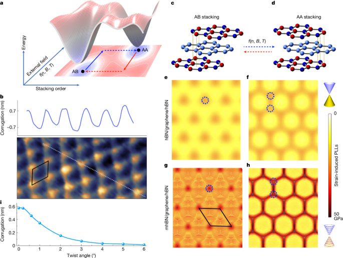
a, Schematic representation of the full phase diagram formed in our double-aligned mhBN/graphene/hBN system. External parameters (such as carrier density n, magnetic field B and temperature T) define one coordinate axis, whereas the intrinsic stacking order of the sandwich heterostructure defines the other. Two local energy minima exist corresponding to AA and AB stacking configurations, with their dominant stackings shown in c and d, respectively. Blue and red arrows indicate transitions between these configurations; solid arrows denote states realized under continuous tuning of external parameters, whereas dashed arrows mark the abrupt structural phase transition, matching the solid and dashed lines in the experiments shown in Fig. 3a–c. b, Moiré-induced corrugation observed in a double-aligned mhBN/graphene/hBN device, measured at room temperature by AFM. Inset shows the corrugation profile along the light blue line. Phonon squeezing reduces corrugation at low temperatures. The unit cell outlined in black matches that in g. c,d, Schematic illustrations of the competing sandwich configurations at double-aligned interfaces: AB (c) and AA (d) stacking configurations. e–h, MD simulations of strain distributions. Panels g and h show our double-aligned mhBN/graphene/hBN configurations with AB and AA stacking configurations, respectively, and panels e and f show reference calculations for double-aligned hBN/graphene/hBN configurations. Comparison highlights the notable role of mhBN on strain enhancement, leading to much stronger reconstruction patterns—triangular and hexagonal reconstructions, respectively. Dashed circles indicate vertices of domains arising from these two reconstruction types, on which strain-induced PLLs develop, as shown on the right. The yellow-to-orange gradient bar indicates increasing strain amplitude. i, The theoretical calculated corrugation of the graphene–hBN interface as a function of the twist angle.
Unlike previous studies that apply a mechanical tool such as an atomic force microscope or scanning tunnelling microscope tip to locally ‘iron’ the sample to toggle the stacking configurations in confined regions of sample27,28, our system allows global, reversible switching between the two stacking states simply by tuning external parameters, including carrier density n, magnetic field B or temperature T. Such all-electronic control is far better suited to device integration and to triggering new phenomena in transport measurements. The schematic in Fig. 1a illustrates the full phase diagram defined by these external parameters and the intrinsic stacking order, in which the two local minima correspond to the competing AB and AA stacking configurations. Accompanying this switch, the moiré-induced strain distribution and thus the lattice reconstruction changes from triangular to hexagonal patterns (Fig. 1e–h; see also the STM images in Fig. 5a,b), ultimately leading to different pseudomagnetic field (PMF) distributions2,29 (Fig. 5e,f) and different band reconfigurations (Fig. 5g–j).
We emphasize that the mhBN is essential for enhancing such lattice reconstruction of graphene, as mhBN itself can accommodate a finite amount of strain, allowing both layers (mhBN and graphene) to undergo very strong relaxation. The molecular dynamics (MD) simulations, comparing mhBN/graphene/hBN (Fig. 1g,h) and hBN/graphene/hBN (Fig. 1e,f) heterostructures, clearly demonstrate that the presence of mhBN greatly amplifies the periodic strain induced by moiré reconstruction. The experimental evidence, including room-temperature atomic force microscopy (AFM) measurement of the corrugation (Fig. 1b) and the same measurement with varying hBN layer numbers (1–4 layers; Supplementary Information Section 13; Supplementary Fig. 19) and their corresponding transport properties, is presented in Supplementary Information Section 4. As well as mhBN, alignment also markedly influences the strain, as shown by the calculated corrugation with respect to the twist angle in Fig. 1i.
Transport device architectures
Two types of transport device are discussed in the main text: dual-gated hBN/graphene/mhBN/hBN (Fig. 2a) and bottom-gated mhBN/graphene/hBN (Fig. 2b). In the former, the mhBN–hBN interface is intentionally misaligned by 15° to achieve superlubricity, preserving the double-aligned sandwich structure. The two architectures are complementary: the dual-gated capped devices enable higher carrier concentrations and allow the roles of doping and the displacement field to be disentangled (Supplementary Information Section 8), whereas the non-capped mhBN/graphene/hBN structure develops stronger reconstruction, in particular the out-of-plane corrugation at the graphene–mhBN interface (Supplementary Information Section 30).
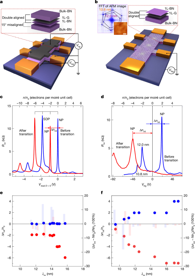
a, Schematic of the transport device with hBN/graphene/mhBN/hBN heterostructure (inset) in a dual-graphite gate configuration. b, Schematic of the mhBN/graphene/hBN transport device. The unencapsulated mhBN enables AFM measurement. Inset, AFM image of the device (bottom right) and its fast Fourier transform (FFT). The FFT confirms the double alignment and gives the periods of both superlattices, which agree well with those derived from the transport measurement in d. Scale bar, 50 nm. c,d, Longitudinal resistance Rxx of the states before (blue) and after (red) the transition in the device types in a and b, measured at T = 1.6 K. The neutrality point, labelled ‘NP’, shifts from no doping to n-doping (device in a) and from p-doping to n-doping (device in b) on transition. The top axis marks doping levels corresponding to integer multiples of electrons or holes per moiré unit cell. The doping shift relative to zero is denoted by Δnint, in which ‘int’ signifies intrinsic doping (in contrast to external doping by gate). For the device in a, the bottom axis (Vdual D = 0) is defined such that both Vtg and Vbg are simultaneously tuned to vary carrier density while maintaining zero displacement field in graphene. By contrast, the device in b has only back gate, so its bottom axis is represented by Vbg. e,f, The doping levels of other same-structured devices with different periods of moiré plaquette λm before (blue dots) and after (red dots) transition. The details of all samples are presented in Supplementary Information Section 3 and Supplementary Figs. 5 and 6. The doping levels of all samples, before and after the transition, are located at integer multiples of electrons per moiré unit cell, with the percentage deviation from ideal integer multiples (Δnint − Nn0)/Nn0 shown by bar graphs at the corresponding positions, in which Δnint − Nn0 is the deviation from the nearest integer multiple N (if N is 0, then we choose the denominator Nn0 = n0).
For both architectures, double alignment of graphene to the hBN crystals on both sides was confirmed by AFM, Raman and transport measurements (Methods; Supplementary Information Section 2). We emphasize that both the double alignment and the presence of mhBN are crucial for the effects we observe, as corroborated by seven types of reference device, none of which exhibit the transition (Methods; Supplementary Information Section 4; Supplementary Figs. 7 and 8).
Integer doping and phase transition
First, let us examine the initial-state transfer curves (blue) of the two device types in Fig. 2c,d. In the hBN/graphene/mhBN/hBN sample, the neutrality point of graphene remains at zero doping, whereas the mhBN/graphene/hBN structure exhibits p-doping. Notably, this p-doping level closely approximates 2n0 (n0 corresponds to doping of one charge carrier per moiré plaquette). In 8 of 9 unencapsulated mhBN/graphene/hBN devices (blue dots in Fig. 2f), the p-doping is quantized at Nn0 (N is an integer between 1 and 4), growing with the moiré period but always fixed at integer multiples of n0.
In Fig. 2e,f, the moiré period, determined from the carrier density of secondary Dirac points, exceeds in many samples the rigid-lattice limit of 14 nm (set by the 1.8% graphene–hBN lattice mismatch) and even reaches 17.7 nm, a consequence of the strain enhancement by mhBN and double alignment19,20 (Methods; Supplementary Information Section 4).
By applying a large positive gate voltage above a certain threshold, a phase transition can be initiated: the moiré period remains unchanged but the samples become n-doped, again by an integer number of electrons per moiré plaquette, for both bottom-gated and dual-gated samples (Fig. 2c,d), and consistently across samples with different moiré sizes (Fig. 2e,f; Supplementary Information Section 3; Supplementary Figs. 5 and 6). Comprehensive control experiments (Supplementary Information Sections 5 and 14; Supplementary Figs. 9–11 and 20–22) verify that this transition and the integer doping are intrinsic, excluding artefacts such as contamination. We emphasize that the integer doping is a direct observation requiring no fitting or registration procedure. As is well established for graphene superlattices5,6,7, the neutrality point–secondary Dirac point separation is fixed at four electrons per moiré unit cell. In Fig. 2c, the post-transition neutrality point (red) falls precisely at the midpoint between the pre-transition neutrality point and the secondary Dirac point (blue) and hence corresponds to exactly two electrons per moiré unit cell, as highlighted by the equally spaced ruler.
Note that for the dual-gated samples (Fig. 2c), the gate voltage was applied simultaneously through top and bottom gates along the D = 0 line30 (dashed line in Fig. 3a). The switching depends only on the total carrier concentration and not on the displacement field (Supplementary Information Section 8; Supplementary Fig. 14). This mechanism fundamentally differs from recently reported two-dimensional ferroelectric systems, in which transitions occur through external electric-field-induced polarization changes26,31,32.
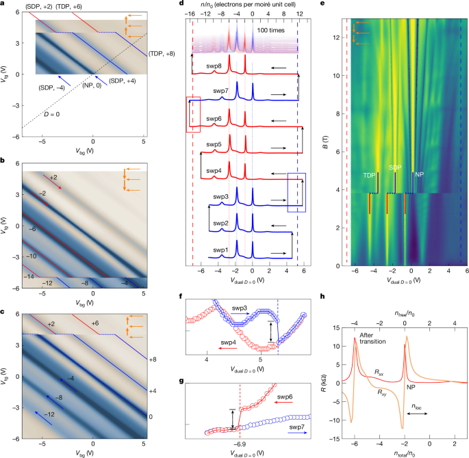
a–c, Vtg–Vbg maps of the transition process, each obtained by sweeping Vbg at stepped Vtg; a–c differ in gate sweep range and sweep history (marked by orange arrows). Orange arrows: sweep directions of top gate (Vtg) and back gate (Vbg). Blue and red arrows or solid lines represent Dirac points before and after transition, respectively. Numbers for blue lines and arrows give the doping per moiré unit cell at neutrality point (NP, 0), secondary Dirac points (SDP, ±4), tertiary Dirac points (TDP, ±8) and quaternary Dirac points (QDP, ±12); numbers for red lines and arrows are the same points offset by −2 electrons. Dashed lines indicate abrupt state changes at transition. The dashed black line in a denotes zero displacement field (D = 0), along which all transfer curves in Figs. 2 and 3 were performed; all forward and reverse transitions in a–c occur on this line, indicating that the displacement field is not the driving mechanism. In a–c, the transition point and the post-transition state are independent of gate range and sweep history. d, Continuous monitoring of the transition. Blue (5.3 V) and red (−6.9 V) dashed lines mark the critical voltages for transition and reversal, respectively. Black arrows track the measurement sequence (swp1–swp8); blue and red denote sweepings starting from the ‘before transition’ and ‘after transition’ states, respectively. Central dashed lines correspond to Δnint/n0 = 0, −4 (blue) and −2 and −6 (red). Shaded region above swp8 represents more than 100 repeated forward/reverse gate sweeps, after which the sample remains unchanged. e, Vdual D = 0–B maps, obtained through Vdual sweeps at fixed magnetic field steps. Orange arrows: sweep and field-variation directions (13 T to 0 T). The Vdual D = 0 sweep range surpasses the critical voltage of the forward transition (dashed blue line at 5.3 V) but not the reverse (dashed red line at −6.9 V) in d. Blue and red solid lines are states before and after transition, respectively. Notably, transition occurs at 3.8 T, at which magnetic length (approximately 13.4 nm) becomes commensurate with moiré periodicity. f,g, Zoom-in views of the blue and red boxed regions in d, respectively, revealing abrupt state changes at critical voltages (dashed lines). Circles represent the plotted resistance points; arrows indicate transition-induced resistance jump. h, Correlation between Rxx and Rxy; top axis, measured Hall density nfree; bottom axis, total gate-induced charge ntotal. The Hall zero-crossing (nfree = 0) occurs at ntotal = 2 holes per moiré cell, the difference being the localized charge nloc.
Transition dynamics
To investigate the transition dynamics and reproducibility, we conducted a series of Vtg–Vbg mappings and repeated switching tests (Rxx in Fig. 3; Rxy in Supplementary Fig. 24). Figure 3a–c reveals several Dirac points separated by intervals of four electrons per moiré plaquette5,6,7, marked with blue (before transition) or red (after transition) lines or arrows.
The phase transition occurs at Vtg = +3.9 V, Vbg = +5.3 V corresponding to ntotal = 3.75 × 1012 cm−2 along the D = 0 line in Fig. 3a. Following the transition, all features shift by two electrons per moiré plaquette. This shift throughout the entire superlattice spectrum clearly indicates that the moiré period is unchanged. The recovery occurs at Vtg = −5.0 V, Vbg = −6.9 V (corresponding to −4.85 × 1012 cm−2), also along the D = 0 line, restoring the entire gate dependence (Fig. 3b). Comparing Fig. 3c with Fig. 3a shows that different Vtg–Vbg ranges and sweep protocols do not affect the transition characteristics: it occurs at identical gate points, as a single discrete event at the critical voltage rather than a continuous evolution.
Figure 3d illustrates the transition dynamics through sequential measurements (swp1–swp8), with dashed lines at +5.3 V and −6.9 V marking the critical voltages for the forward and reverse transitions, respectively. Below the critical voltage, no transition occurs (swp1–swp2); on reaching it, the transition happens (swp3–swp4), at a critical voltage independent of the gate sweep rate (Supplementary Information Section 15; Supplementary Fig. 23). Similar behaviour is observed for the reverse transition (steps swp4–swp7). Figure 3f,g shows zoomed-in views around the critical voltages for both the forward and reverse transitions. At the moment of transition, the resistance jumps from one state to another without any intermediate states, consistent with the abrupt translation of features observed in Vtg–Vbg mappings of Fig. 3a–c. Once the transition is induced, further increasing the gate voltage yields no continuous effect, indicating a saturation mechanism defined by the moiré unit cell capacity rather than the strength of the applied field. This behaviour differs markedly from that of ferroelectrics, for which polarization scales continuously with the applied field. The switching is fully reproducible: 100 consecutive cycles yield curves that overlap precisely (Fig. 3d, top). All behaviours discussed above support that the observed phase transition is a first-order-like transition (further information in Supplementary Information Section 43).
Notably, the transition can also be controlled by the magnetic field. Mapping the transition from 13 T down to 0 T (Fig. 3e) shows that the transition is suppressed at high field, even for gate voltages far exceeding the critical value, and reappears at exactly the same critical voltage once the field drops below Bcrit = 3.8 T. The origin of this suppression remains to be established; we note, however, that the magnetic length at critical field \(\sqrt{\hbar /e{B}_{{\rm{crit}}}}\approx 13.4\,{\rm{nm}}\) is comparable with the moiré period for this sample of 13.8 nm.
In Fig. 3h, correlating Rxx with Rxy gives further information for theoretical analysis: the Hall-resistivity zero crossing (zero free carrier density nfree) occurs at a gate-induced density of two holes per moiré unit cell, the difference being compensated by localized electrons nloc.
Origin of the phase transition
To identify the origin of the phase transition, we consider the balance between elastic (strain) and van der Waals forces5,6, which can be modified through Coulomb interactions introduced by gate charging the graphene layer.
Using high-throughput density functional theory (DFT), we calculated the adhesion-energy distribution across the non-relaxed moiré plaquette, assuming perfect alignment of hBN on both sides, for the AB (Fig. 4a) and AA (Fig. 4b) relative configurations of the two hBN crystals (Supplementary Information Section 22; Supplementary Figs. 33–35). The relative energy of the two configurations can be compared by averaging the van der Waals potential over the entire moiré unit cell, as illustrated in Fig. 4c. The AB structure exhibits lower energy under neutral charging conditions (Fig. 4c–e). However, by assigning a negative charge on graphene above a certain threshold (corresponding to positive gate voltage applied) the AA configuration becomes more energetically favourable than AB (Fig. 4c,f,g), resulting in a structural phase transition from AB to AA.
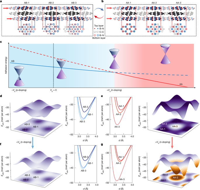
a,b, Schematics of the two configurations (AB (a) and AA (b)) and three high-symmetry stacking sites for both configurations. The red arrows on the left side indicate a shift of one of the hBN layers by one interatomic distance. c, Schematic diagram of the relative stability (in terms of the average adhesion energy taken over the entire moiré plaquette) of the two configurations as a function of doping. The solid lines represent the energy-favourable state. The crossing of the blue and red lines indicates the occurrence of the transition. Electron doping (positive gate) switches the relative stability between the two configurations and the consequent modification of the interlayer adhesion is proposed to be the driving force. d–g, Distribution of the interlayer adhesion energy (Eadh) across the moiré plaquette for the AB (d,f) and AA (e,g) configurations in the case of zero (d,e) and n-type (f,g) external doping (induced by gating in our experiments). The graphs in the middle give the corresponding adhesion energies of the three high-symmetry stackings as a function of interlayer distance between graphene and the top and bottom boron nitride layers near the equilibrium spacing (2.7–4.0 Å).
The energy evolution with doping arises from gate-introduced Coulomb interactions, which enter the competition between van der Waals forces and elastic energies5,6. The balance among these three factors can be understood by comparing the relative stability of the AB and AA stacking configurations at high-symmetry points (Fig. 4a,b), which are the most representative sites and capture the qualitative trends under gating. Specifically, n-type doping substantially reduces the interlayer potential of AA-3 stacking: there, carbon atoms are vertically aligned with boron and the added electrons on carbon are strongly attracted to the positive charge on boron arising from the ionic nature of B–N bonds33. By contrast, the interlayer potential of AA-2 stacking is slightly elevated by the repulsion between the added electrons and the negatively charged nitrogen, whereas AA-1 and all three high-symmetry sites of the AB alignment remain almost unchanged, as the interaction of added electrons with boron is compensated by their interaction with nitrogen. This picture is substantiated by DFT calculations (Fig. 4d–g; Supplementary Information Sections 22–27). We can generalize the similar gate-induced phase transitions to other systems in which at least one of the multiply aligned layers has electropolarity (Supplementary Information Section 37).
Origin of integer doping
We now turn to the origin of the integer doping in graphene, which we attribute to strain-induced PLLs localized at the vertices of the reconstructed moiré domains. The reconstructed phases for AB and AA configurations are directly visualized through STM measurements (STM images of different regions, and of a reference single-aligned graphene/hBN region on the same flake, are shown in Supplementary Figs. 12 and 13) and theoretically simulated by MD calculations (Fig. 5a,b). On the basis of the atomic displacements calculated by MD, we obtained the strain distribution in the reconstructed moiré unit cell (schematics shown in Fig. 5c,d), as well as the associated pseudomagnetic field7,8,9,10,11,34 (left panels of Fig. 5e,f) (Supplementary Information Sections 24, 29 and 31).
The reconstruction results in distinct strain fields for the AB and AA configurations (Fig. 5c,d). For the AB configuration, it is the AB-1 and AB-3 stackings that have much lower energy than AB-2 (Fig. 4d,f), so the reconstruction forms triangular domains of AB-1 and AB-3 stackings, accompanied by notable strain and out-of-plane corrugation at the AB-2 stacking (Fig. 5c). By contrast, for the AA configuration, it is the AA-3 stacking that has the lowest energy (Fig. 4e,g), leading to hexagonally reconstructed AA-3 moiré domain, with the strain concentrated at AA-2 and AA-1 stacked corners of the moiré plaquette (Fig. 5d). Here the predominance of in-plane strain in AA (versus out-of-plane corrugation in AB) originates from the mirror symmetry of the AA configuration, which yields negligible net out-of-plane force (Supplementary Information Section 38; Supplementary Fig. 54). In both cases, the strain results in strong PMF.
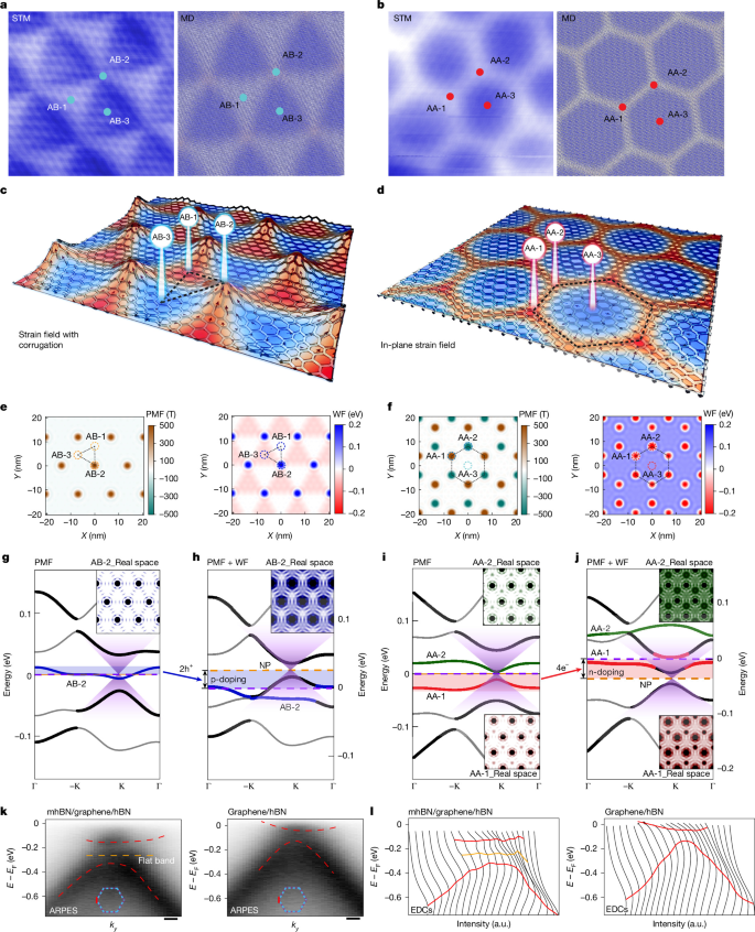
a,b, Left panels, STM images of the AB (a) and AA (b) configurations. Right panels, corresponding MD simulations (details in Methods and Supplementary Fig. 36). Both STM images and MD simulations confirm strong reconstruction: triangular in AB (a) and hexagonal in AA (b). c,d, Schematic illustrations of the strain distribution in the reconstructed AB (c) and AA (d) configurations. Background colour: relative strain magnitude; semi-transparent hexagonal lattice: deformation of the graphene lattice under the forces indicated by arrows. In AB (c), strain is dominated by out-of-plane corrugation, strongest at AB-2. In AA (d), in-plane forces compress the AA-1 and AA-2 stackings and expand AA-3. e,f, The PMF (left panels) and work function (WF, right panels) reveal one pinch point in AB (e) and two in AA (f). The WF contrast between pinch points and the bulk regions is opposite for AB and AA. These distributions, from MD and DFT calculations, are the input for the band structures in g–j. g–j, The band structure calculated from the effective model without (g,i) and with (h,j) the WF considered. Flat bands (bandwidth 24 meV in AB and 17 meV in AA) originating from the localized states at the pinch points are shown in bold colours; Dirac-cone-derived bands in bold black. With WF included, the flat bands shift down (AB, h) or up (AA, j), crossing the dispersive bands. Dashed purple lines mark the Fermi level, dashed orange line marks the neutrality point (NP) and black arrows indicate the gap between them. Blue and red shading are the integer numbers of holes and electrons transferred between flat and dispersive bands. Insets, real-space density distributions of the correspondingly coloured bands. k,l, ARPES spectra (k) and energy distribution curves (EDCs) (l) of double-aligned mhBN/graphene/hBN and its reference graphene/hBN, measured along the momentum cuts indicated by the red lines in the Brillouin zone diagrams in k. Dashed red curves, dispersive features from EDC fits, arising from band folding induced by graphene–hBN alignment. Dashed orange line, guide to the flat band from EDC fits, attributed to PLLs. Scale bars, 0.02 Å−1. a.u., arbitrary units.
The effect of this strong reconstruction on the band structure involves two ingredients: (1) the PMF and (2) variations of the local work function across the moiré plaquette35. We first calculated the band structure for the reconstructed AB and AA configurations, excluding the variations in work function (Fig. 5g,i). Two features emerge: (1) a substantial bandgap is opened owing to the reconstruction-induced difference between the on-site potential of each carbon sublattice35,36,37; (2) several fourfold spin-valley degenerate flat bands appear within the bandgap (Supplementary Information Sections 29, 31 and 32). Plotting the corresponding real-space wavefunctions (inset colour maps in Fig. 5g,i) reveals their localization at the vertices of the moiré domain AB-2, AA-1 and AA-2, in which strain and the PMF both peak. These flat bands can be interpreted as PLLs arising from the PMF. In reciprocal space, they are manifested as flat bands that host strongly localized electrons25. Equivalently, we can view them as strain-induced quantum dots situated at the moiré-domain vertices. Notably, because the zeroth PLL in graphene sits at the NP and is only half-filled, it cannot change the doping level unless its energy is shifted and hybridizes with either the valence or the conduction dispersive bands.
Taking into account the work-function landscape across the moiré plaquette (owing to local strain and van der Waals environment) shifts the flat bands away from the bandgap, hybridizing them with either the valence or the conduction bands and thus resulting in doping of graphene. The curvature at the AB-2 site lowers the hybridization of the pz orbital of carbons (similar to carbon nanotubes38), increases the local work function at AB-2 and consequently shifts its corresponding flat band downward (Fig. 5h). Conversely, the in-plane strain at AA-1 and AA-2 vertices reduces the carbon–carbon distance, resulting in the reduction of the local work function and upward shift of the corresponding flat bands39 (Fig. 5j). Other factors, such as the van der Waals environment, contribute with the same trend35,37 (Supplementary Information Section 27; Supplementary Figs. 43–45).
The resulting work-function variation lowers the flat bands towards the valence band in the AB configuration and raises them towards the conduction band in AA (Fig. 5h,j). Once the empty/filled flat bands in the AB/AA configuration cross the valence/conduction band, the holes/electrons trapped in the corresponding quantum dots are released into the body of the moiré domain and start to contribute to transport. This shifts the Fermi level away from the neutrality point to the valence/conduction bands and the AB/AA configuration will demonstrate p-doping/n-doping, respectively. In this picture, electrons are redistributed between the conductive moiré domain and the insulating quantum dots at its vertices.
Hole-side angle-resolved photoemission spectroscopy (ARPES) measurements corroborate this picture. Comparing the mhBN/graphene/hBN heterostructure against a conventional graphene/hBN reference region on the same flake (Fig. 5k,l), a flat band (orange) appears exclusively in the mhBN region and hybridizes with the neighbouring dispersive band (red), consistent with our above picture.
Such a doping mechanism explains the observed integer charging per moiré plaquette. In the simplest picture, each PLL holds g = gsgv = 4 states (spin × valley degeneracy). In the AB configuration (Fig. 5e), this condition is met at only one vertex per plaquette. Because the zero-energy PLL is initially half-filled, each vertex accommodates two more electrons (or holes), giving n/n0 = +2 for the initial p-doped state (blue sweep in Fig. 2d); in the AA configuration, two vertices contribute, giving n/n0 = −4 (red sweep). This accounts for the p-doping before the transition being consistently smaller than the n-doping after it.
Building on the above simplest picture, understanding such integer quantization also requires fundamental energy balance considerations. A well-established physical principle for structural stabilization seen in phenomena ranging from the Peierls transition in one-dimensional crystals to the filled shells of noble gases is as follows: when energy spectra are discrete, configurations with fully occupied and fully empty states separated by a gap become energetically favoured. In our system, the necessary discrete spectrum arises not from atomic orbitals or external magnetic fields but from PLLs generated by the strong periodic strain of the moiré reconstruction. Crucially, this solid-state system has a tunability absent in atomic prototypes: it can tune the electrostatic energy directly by solid gate and self-optimize the energy spectrum to maintain integer fillings. Similar to flux optimization in GaAs quantum rings40, the system can adjust the PMF strength (through strain redistribution) to ensure that the PLL degeneracy exactly matches the electron occupancy. The finite energy gain from fully occupying a Landau level compensates for the extra elastic deformation costs, effectively locking the system into a stable, integer-quantized state. We note that this self-optimization operates at the local scale involving only small strain variations around moiré vertices. This local self-optimization is distinct from the global structural transition itself, which is driven by the competition between van der Waals, elastic and electrostatic energies (Fig. 4).
Further evidence identifying commensurate filling of the discrete PLL spectrum as the origin of the integer doping, and ruling out alternative scenarios (charge trapping, Coulomb blockade of moiré-potential quantum dots, interfacial ferroelectricity and contact electrostatics), is provided in Supplementary Information Section 39.
Outlook
We believe that our work opens a new avenue for engineering structural and electronic phase transition in dynamical van der Waals systems through careful balancing of Coulomb, van der Waals and elastic energy contributions. Structures with several aligned interfaces can result in more complex phase transitions and electronic states. We also point out that the periodic arrangement of localized PLLs demonstrated here constitutes a regularly distributed array of quantum dots defined by strain. This connection to quantum dot physics opens avenues for further fundamental and applied investigations. Notably, such integer doping and phase transition occur across a broad range of moiré sizes (from 6 nm to 17.7 nm), eliminating the requirement for precise twist angle control in sample fabrication.
Methods
Device fabrication
Heterostructures were assembled using the standard dry-transfer technique. Two device architectures were used: dual-gated hBN/graphene/mhBN/hBN, in which the mhBN–hBN interface was intentionally misaligned by 15° to ensure superlubricity, and bottom-gated mhBN/graphene/hBN. Seven more types of reference device were fabricated by the same process (full list and data in Supplementary Information Section 4). The sample types are categorized by alignment and hBN thickness. The alignment scenarios include double alignment (a), single alignment (b), top and bottom hBN aligned with each other but not with the encapsulated graphene (c), single alignment with unencapsulated graphene (d) and a nonaligned three-layer stack (e). Samples with the same alignment are further subdivided by hBN thickness (bulk, bilayer and monolayer hBN), as illustrated in the schematics in Supplementary Fig. 7, into a1–a4, b1, b2, c1, d1 and e1. The a2 and a4 samples are the devices used in Fig. 2, listed in Supplementary Tables 1 (samples 1–8) and 2 (samples 9–10). Other sample types are for reference with data in Supplementary Information Section 4.
Confirmation of double alignment and mhBN
For the non-capped (single-gated) samples, simultaneous alignment of graphene to both hBN crystals was confirmed by AFM and transport measurements: the Fourier transform of the AFM topography (inset of Fig. 2b) shows two moiré periodicities of 10.8 nm and 12.0 nm (ref. 19), corroborated by the two sets of secondary Dirac points in the transfer curves13,14,15,41 (Fig. 2d). For the dual-gated encapsulated samples, in which the two moiré patterns are practically identical in size and the secondary Dirac points coincide in gate voltage, double alignment was confirmed primarily by Raman spectroscopy combined with optical imaging and AFM (ref. 42). Detailed analysis is given in Supplementary Information Section 2. The thickness of the hBN layers (down to monolayer) was confirmed by Raman and AFM measurements (Supplementary Information Section 2).
Transport measurements
Transport measurements were performed in a TeslatronPT cryostat at a base temperature of T = 1.6 K, equipped with a superconducting magnet providing fields up to 14 T. Longitudinal and Hall resistances were measured in a four-terminal configuration using standard low-frequency lock-in SR860 lock-in amplifiers, with an AC excitation current of 5 nA at 37 Hz to avoid sample heating. Gate voltages were applied by a Keithley 2601 source meter. For dual-gated devices, the top-gate and back-gate voltages were swept simultaneously along the D = 0 line30 unless stated otherwise. The critical transition voltage is independent of the gate sweep rate (Supplementary Information Section 15); control experiments excluding contamination and other artefacts are detailed in Supplementary Information Sections 5 and 14.
DFT calculations
The stability, work function, electronic structures and charge transfer of the hBN/graphene/hBN heterostructures have been thoroughly studied using DFT calculations. Our calculations are based on the Perdew–Burke–Ernzerhof functional as implemented in the Vienna Ab Initio Simulation Package (VASP). The interaction between the valence electrons and ionic cores is described within the projector augmented-wave approach with a plane-wave energy cut-off of 500 eV. The widely used semi-local approximations for the exchange-correlation energy do not take long-range correlations into account correctly. Thus, they fail to reproduce van der Waals attraction and the prediction of equilibrium geometries of van der Waals bound layered systems. To address the issue, the dispersion correction schemes proposed by Grimme were used to treat the interlayer interaction between graphene and hBN layers. The Brillouin zone was sampled with the Monkhorst–Pack grid and the grid sizes depend on the size of the supercells used. The grid was chosen to be as dense as 31 × 31 × 1 for a primitive cell and Γ-point only for a large supercell of near 5 nm. The vacuum space of at least 15 Å was used to avoid interaction between neighbouring layers. In the structural energy minimization, the atomic coordinates are allowed to relax until the forces on all of the atoms are less than 0.01 eV Å−1. The energy tolerance is 10−6 eV.
Because full-scale DFT calculation would be computationally unrealistic for a moiré unit cell consisting of 56 × 56 atoms of graphene monolayer and at least twice the 55 × 55 atoms of two hBN layers, we would investigate the structure using a combination of DFT calculations and empirical potentials MD simulations. For specified stacking of the hBN/graphene/hBN heterostructures, calculations were done using the commensurate structure with the graphene lattice. To understand the adhesion energy and the work function distribution of the moiré structure, we screen the local stacking of the moiré cell of hBN/graphene/hBN using a 21 × 21 grid of sampling points. The structure at each sampling point was obtained by shifting the graphene with respect to the hBN layers on the two sides. To model the gate-induced electron doping in graphene, extra electrons were added to the supercell and a uniform positive charge background was added to compensate and ensure the charge neutrality of the system.
MD simulations
The structure relaxations were implemented in the Large-scale Atomic/Molecular Massively Parallel Simulator (LAMMPS). We used many-body Tersoff potentials to treat the in-plane C–C and B–N interactions. The interlayer van der Waals interaction between the graphene and hBN was described by the registry-dependent Kolmogorov–Crespi potential. To model the interlayer interaction between graphene and hBN under gating, we vary the strength of the C–B interaction relative to the C–N interaction using a scaling parameter (s). We found that, for s = 5% and s = 50%, the potential is qualitatively consistent with the DFT interlayer adhesion of the trilayer heterostructure in the absence and presence of doping, respectively. Using the s = 50% scaling of the C–B/C–N interaction, we successfully simulated the structural transition of the heterostructure. To include the substrate effect of bulk hBN and model the interlayer interactions among different boron nitride layers, we proposed a Lennard–Jones 6–12 potential to describe the repulsive and attractive terms, and Coulomb’s law is used for the electrostatic interactions. This yields
in which ϵij and σij are the potential parameters to control the strength of the attractive and repulsive interactions, respectively, rij is the interaction distance between atom i and atom j, qi and qj are the atomic partial charge in units of the elementary charge and Kc is the coulombic constant. We set 0.2 and −0.2 for the B and N, respectively after careful evaluation. Because of the smaller van der Waals radius of B (about 1.92 Å) and large interlayer distance of hBN layers (about 3.30 Å), we neglected the short-range B–B interactions in this study. ϵBN and ϵNN were set to 0.3035 and 10.8237 meV, respectively. Also, we used 3.75 and 3.1461 Å for σBN and σNN, respectively. During the simulation, the cut-off distance was set to 8 Å for the attractive and repulsive terms. A long-range solver of the standard coulombic Ewald summations was used to compute long-range coulombic interactions or long-range interactions. The atomic structures were equilibrated using the NVT ensemble (canonical ensemble). A 2.0-ns annealing process from 300 K to 1 K was first carried out and then the other 0.5-ns timescale was implemented to stabilize the structures. A time step of 1.0 fs was used and the relaxation was completed when the forces are less than 10−6 eV Å−1. The unrotated heterostructures were modelled by 56 × 56 unit cells of graphene and 55 × 55 unit cells of hBN, resulting in a 1.8% mismatch in lattice constant. We used four monolayers of hBN to imitate bulk substrate, in which the bottom two layers were fixed and the top two layers allowed relaxation during the MD simulations.
Continuum model calculations
The lattice structures of graphene and hBN are incommensurate; although both feature a honeycomb lattice (graphene of carbon atoms and hBN of boron and nitrogen atoms), the hBN lattice period is δ ≈ 1.8%, longer than that of graphene, a = 0.246 nm. Including an anticlockwise twist of the hBN layer, θ, the interference of the two lattice potentials at the interface gives a moiré superlattice, magnified from the graphene lattice, with moiré superlattice period \(\lambda \approx a/\sqrt{{\delta }^{2}+{\theta }^{2}}\), and rotated by φ ≈ −arctan(θ/δ). The moiré superlattice Bragg vectors are constructed as linear combinations of the ‘first star’ of non-zero vectors, Gm ≈ δ · gm − θ(ez × gm) m = (0, 1,…, 5), expressed in terms of the first star of graphene vectors, \({{\bf{g}}}_{{\rm{m}}}=\frac{4\pi }{\sqrt{3}a}\left(-\sin \frac{m2\pi }{3},\cos \frac{m2\pi }{3}\right)\), and depicted alongside the moiré Brillouin zone.