 Newshot
Main
Analogue simulation offers insights into quantum field theories pertaining to phenomena in naturally inaccessible settings, such as the early Universe. Time evolution in a quantum-field-theory simulator is especially valuable owing to the computational complexity of non-perturbative many-body dynamics. Single-component atomic Bose–Einstein condensates, with tunable microscopic Hamiltonians, provide a simulation platform for massless relativistic fields and have been used to simulate cosmological acoustic fluctuations20,21,22,23,24,25. Extending experiments to two-component Bose–Einstein condensates with coherent inter-component coupling4,5,26,27,28,29,30, one can simulate quantum field theories with massive fields and compact conjugate variables, which can display long-wavelength non-perturbative dynamics31,32,33,34,35,36,37,38,39,40,41,42,43 and support broader families of topological defects8,10,44. In particular, this allows realization of the paradigmatic sine-Gordon model8 for massive relativistic fields. Previously, this was achieved in d = 1 dimension31,32,34,35,37,40, where the model (for a uniform system) is integrable9. Here we realize analogue simulation of massive relativistic quantum fields in d = 2 and observe both perturbative and non-perturbative sine-Gordon dynamics.
Our simulator is based on a coherently coupled mixture of two miscible hyperfine states of 39K atoms in a two-dimensional optical box trap6,7,45; we denote the two states \(|\uparrow \rangle \) and \(|\downarrow \rangle \), and their individual wavefunctions \({\psi }_{\uparrow ,\downarrow }=\sqrt{{n}_{\uparrow ,\downarrow }}{{\rm{e}}}^{-i{\phi }_{\uparrow ,\downarrow }}\), where n↑,↓ and ϕ↑,↓ are densities and phases of the individual components. In our gas, the two-dimensional total density n = n↑ + n↓ is essentially uniform, but the spin state varies in space (Fig. 1a); on the Bloch sphere, the two compact conjugate variables are the local population imbalance Z(x, y) = [n↑(x, y) − n↓(x, y)]/[n↑(x, y) + n↓(x, y)] and the relative phase of the two components ϕ(x, y) = ϕ↑(x, y) − ϕ↓(x, y). In general, the spin dynamics depend on both the strength of the coherent coupling, given by the Rabi frequency Ω, and the spin-dependent nonlinear interactions. The latter are characterized by a parameter μs that has a similar role to a chemical potential (Methods), for example, setting the spin sound speed c. In the Josephson regime, μs ≫ ħΩ (where ħ is the reduced Planck constant), fluctuations in Z are strongly suppressed, and long-wavelength spin dynamics are dominated by fluctuations in ϕ. At constant Z, the energy cost for ϕ to deviate from 0 (defined by the Rabi vector) corresponds to a potential \(U(\phi )=-(\hbar \varOmega /2)\cos \phi \) (Fig. 1b), which leads19 to the sine-Gordon equation
with \(c=\sqrt{{\mu }_{{\rm{s}}}/m}\), where m is the atom mass, and the field mass \({m}^{* }=m\sqrt{2\hbar \varOmega /{\mu }_{{\rm{s}}}}\), which arises from the coherent coupling that breaks the U(1) symmetry of ϕ. Solutions of this model include domain walls where ϕ rapidly winds by 2π (refs. 8,10,44). Whereas in d = 1 such walls are just point defects, in d > 1 they are extended objects that can exhibit non-trivial patterns13,14.
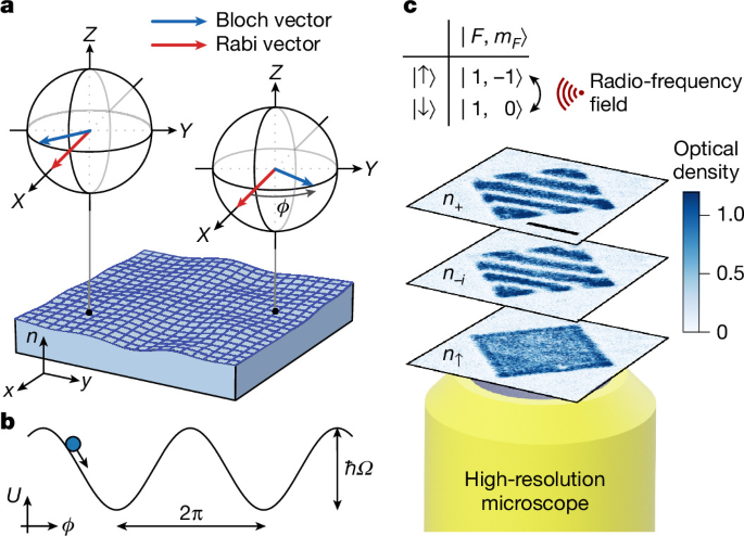
a, The concept. In our two-dimensional Bose–Einstein condensate, the density n is essentially uniform, and we use a spatially varying spin state, shown by the Bloch vectors, to encode a massive relativistic field. The conjugate variables Z(x, y) and ϕ(x, y) are, respectively, the local population imbalance and relative phase of spin components \(|\uparrow \rangle \) and \(|\downarrow \rangle \), which are coherently coupled by a radio-frequency field, indicated by the Rabi vector. b, The sine-Gordon model. In the Josephson regime, μs ≫ ħΩ, where μs is the characteristic interaction-energy scale for the spin degrees of freedom and Ω is the radio-frequency Rabi frequency, ϕ evolves under a sinusoidal potential U. c, The experiment. Our \(|\uparrow \rangle \) and \(|\downarrow \rangle \) are two hyperfine states of 39K. We image both the local populations n↑,↓ = ∣ψ↑,↓∣2 (where ψ↑,↓ are the wavefunctions) and the transverse spin projections n+,− = ∣ψ↑ ± ψ↓∣2/2 and ni,−i = ∣iψ↑ ± ψ↓∣2/2. Here we show example images of n+, n−i and n↑, for a cloud with uniform n and Z but a magnetically imprinted linear ϕ gradient. Scale bar, 20 μm.
In our experimental set-up (Methods), \(|\uparrow \rangle =|1,-1\rangle \) and \(|\downarrow \rangle =|1,0\rangle \) in the \(| F,{m}_{F}\rangle \) basis; here F denotes the total angular momentum and mF its projection along the quantization axis. We couple the two spin states by a radio-frequency field with Ω up to 2π × 20 kHz. With our magnetic field (B) stability of approximately 150 μG, our error in the radio-frequency detuning δ is δerr ≈ 2π × 100 Hz. The contact interactions between atoms in states \(\sigma ,{\sigma }^{{\prime} }\in \{\uparrow ,\downarrow \}\) are characterized by parameters \({g}_{\sigma {\sigma }^{{\prime} }}\propto {a}_{\sigma {\sigma }^{{\prime} }}\), where \({a}_{\sigma {\sigma }^{{\prime} }}\) are s-wave scattering lengths. We operate near B = 58 G, where a↑↑ ≈ 32 a0 and a↑↓ ≈ −53 a0 (where a0 is the Bohr radius) are essentially constant, and a↓↓ is tunable via a Feshbach resonance. We tune a↓↓ > 85 a0 to ensure that \({a}_{\uparrow \uparrow }{a}_{\downarrow \downarrow } > {a}_{\uparrow \downarrow }^{2}\), so that the mixture is miscible and stable against mean-field collapse46. In our experiments, n ≈ 102 μm−2 and μs = κn ≈ 2πħ × 800 Hz, where κ = (g↑↑ + g↓↓ − 2g↑↓)/4. We start our experiments with a quasi-pure condensate; from our trap depth of approximately kB × 30 nK (where kB is the Boltzmann constant), we estimate the temperature to be ≲10 nK, whereas the Berezinskii–Kosterlitz–Thouless critical temperature corresponding to our n is TBKT ≈ 0.5 μK (ref. 47).
Using in situ state-selective absorption imaging (Fig. 1c), we directly image n↑,↓(x, y) = ∣ψ↑,↓(x, y)∣2. By applying suitable π/2 spin rotations48, just before the imaging, we can also measure n+,−(x, y) = ∣ψ↑ ± ψ↓∣2/2 or ni,−i(x, y) = ∣iψ↑ ± ψ↓∣2/2. In addition, to measure projections of the global Bloch vector (X, Y or Z), averaged over the system, we (after any necessary π/2 rotations) release the atoms from the trap, spatially separate \(|\uparrow \rangle \) and \(|\downarrow \rangle \) components with a Stern–Gerlach gradient and image them simultaneously.
For general \({g}_{\sigma {\sigma }^{{\prime} }}\), spin-dependent interaction energy is minimized for Z = Z0, where Z0 = −Δ/κ, with Δ = (g↑↑ − g↓↓)/4 (Methods). For Z = Z0, the interaction contribution to the chemical potentials of the two components, μ↑ and μ↓, is equal. Consequently, total-density fluctuations do not change μ↑ − μ↓, and thus (to leading order) do not couple to the spin dynamics19, which is essential for realizing the sine-Gordon model in the spin sector. It is noted that Z0 = 0 for a \({{\mathbb{Z}}}_{2}\)-symmetric system (Δ = 0), whereas in our case Δ < 0, so Z0 > 0.
In Fig. 2, we show how we initialize our simulator at Z0, for different Z0 values. In one scenario, we first use strong radio-frequency coupling to adiabatically rotate the Bloch vector from state \(|\uparrow \rangle \) to the theoretically predicted Z0. Then, as we slowly (over 10 ms) reduce the radio-frequency coupling to reach the Josephson regime, Z remains constant; see (1) in Fig. 2a and open symbols in Fig. 2b. Here we proportionally reduce Ω and δ, so that the Rabi vector (Ω, 0, δ) remains aligned to Z0. Alternatively, if we instead prepare a strongly coupled symmetric mixture (Z = δ = 0) and then slowly reduce Ω, the interactions ‘torque’ the Bloch vector towards Z0; see (2) in Fig. 2a and solid symbols in Fig. 2b. Remarkably, one does not need to know the correct Z0 a priori—the system spontaneously and robustly finds it as the ground state in the Josephson regime.
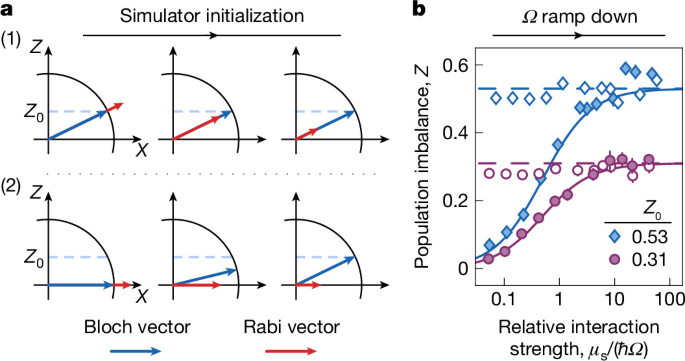
a, Experimental protocols. Spin and total-density dynamics decouple for Z = Z0 (see text). In protocol (1), we prepare the system at the predicted Z0 using strong radio-frequency coupling, and then reduce this coupling to reach the Josephson regime, μs ≫ ħΩ. Alternatively, in (2), we start with a strongly coupled symmetric mixture (Z = 0) and, as we reduce Ω, a non-zero Z spontaneously emerges and tends towards Z0. b, Experimental data for protocols (1) (open symbols) and (2) (solid symbols), for two sets of interaction parameters corresponding to different Z0 values (Methods). The dashed lines show the predicted Z0 and the solid lines show predictions based on \(\chi ={\rm{d}}Z/{\rm{d}}\delta \approx {[\varOmega +2{\mu }_{{\rm{s}}}/\hbar ]}^{-1}\), where δ is the radio-frequency detuning; for the same Ω, the radio-frequency field in protocol (2) is detuned from that in (1) by −Z0Ω, so Z ≈ Z0(1 − χΩ). Each data point is based on ten independent experimental runs; the symbols show the mean values and the error bars (often smaller than symbol sizes) denote the s.e.m.
This robustness also highlights an experimentally important reduced sensitivity to δerr. In a non-interacting system, spin control with error Zerr ≪ 1 requires δerr ≪ Ω, which can pose challenging demands for the B-field stability30. However, here, interactions reduce the magnetic susceptibility \(\chi ={\rm{d}}Z/{\rm{d}}\delta \approx {[\varOmega +2{\mu }_{{\rm{s}}}/\hbar ]}^{-1}\) (refs. 5,49), so Z is robust as long as δerr ≪ 2μs/ħ, and we achieve Zerr < 0.07 (root mean square) even for δerr ≫ Ω.
In Fig. 3, we examine the global spin dynamics in our system, for Z0 = 0.31. By jumping the phase of the radio-frequency field (which defines ϕ = 0), we globally displace the Bloch vector and excite plasma oscillations (Fig. 3a), such as seen in Fig. 3b.
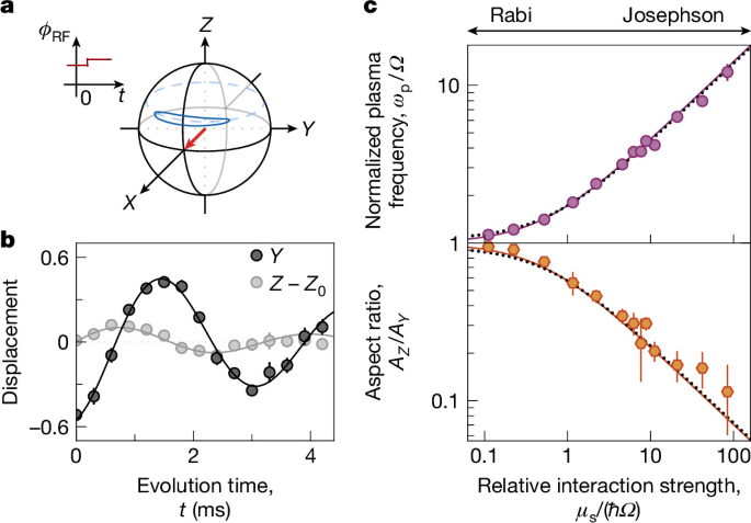
a, A jump in the radio-frequency-field phase, ϕRF, initiates global spin oscillations. Interactions squash the oscillation trajectory (blue ellipse) in the Z direction. b, An example of Y and Z oscillations, for μs/(ħΩ) ≈ 11; here ϕ ≈ Y. Damped-sine fits (solid lines) give the plasma frequency ωp and the oscillation amplitudes AY and AZ < AY. Each data point is based on five independent experimental runs; the symbols show the mean values and the error bars (often smaller than the symbol sizes) denote the s.e.m. c, Dependence of ωp/Ω and AZ/AY on μs/(ħΩ). The Rabi and Josephson regimes, respectively, correspond to μs/(ħΩ) ≪ 1 and μs/(ħΩ) ≫ 1. For the measurements here, Z0 = 0.31, and the dotted lines show the corresponding theoretical predictions (Methods), whereas the essentially indistinguishable solid lines show the predictions for Z0 = 0 from equations (3) and (4). The error bars show fitting errors.
Here, neglecting small corrections due to Z0 not being zero (Methods), the displacements δZ and \(\delta Y\approx \sin \delta \phi \approx \delta \phi \) evolve under the effective Lagrangian density
The energy cost of a ϕ displacement is only due to U ∝ ħΩ, but the cost of a Z displacement also includes an interaction-energy penalty, ∝ μs. The ratio of these costs gives the ratio of the oscillation amplitudes:
and their product gives the plasma-oscillation frequency
In the non-interacting (Rabi) limit AZ = AY and ωp = Ω, and in the Josephson regime AZ ≪ AY, which is essential for the implementation of the sine-Gordon model, and \(\hbar {\omega }_{{\rm{p}}}\approx \sqrt{2\hbar \varOmega {\mu }_{{\rm{s}}}}\gg \hbar \varOmega \) is the mass gap m*c2 in equation (1).
Our measurements (Fig. 3c) agree with the predictions of equations (3) and (4) over three orders of magnitude in μs/(ħΩ). Crucially, we observe coherent oscillations deep in the Josephson regime, up to μs/(ħΩ) ≈ 102.
Next, we turn to the finite-momentum (k > 0) spin excitations (Fig. 4). By modulating Ω at frequency ωm, we parametrically excite finite-k spin modes with frequency ωs(k) = ωm/2 (Fig. 4a). It is noted that the coupling of this parametric drive to the total-density modes is much weaker. Figure 4b shows example images with and without parametric modulation. We measure n−i(x, y), which reveals the ϕ excitations. For every ωm, we observe ϕ modulations with a well-defined spatial frequency k, and thus map out the spin dispersion relation, shown in Fig. 4c for different m* values.
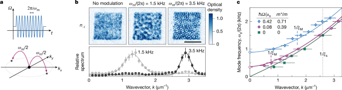
a, Experimental protocol. We parametrically excite the system by modulating Ω at frequency ωm. The injected energy, in quanta of ħωm, is converted to pairs of spatial excitations with opposite momenta, each carrying energy ħωm/2. b, Example measurements. Top: after the parametric modulation, images of n−i show fluctuations with a characteristic ωm-dependent length scale. Scale bar, 20 μm. Bottom: normalizing the spatial power spectrum of the fluctuations observed with modulation to that without modulation, we reveal the dominant k excited at each ωm, which gives ωs(k) = ωm/2. Each data point is based on five independent experimental runs; the symbols show the mean values and the error bars denote the s.e.m. The solid lines show Gaussian fits. c, Dispersion relations for different field masses m, tuned by varying the value of Ω (around which we modulate); here we also include k = 0 plasma-oscillation measurements. The solid lines show theoretical predictions from equation (5). The dashed lines indicate the inverse magnetic healing lengths \(1/{\xi }_{{\rm{M}}}=\sqrt{2m\varOmega /\hbar }\); in our system, ξM corresponds to the reduced Compton wavelength ħ/(mc). The dotted line shows the inverse spin healing length, \(1/{\xi }_{{\rm{s}}}=\sqrt{2m{\mu }_{{\rm{s}}}/{\hbar }^{2}}\), which sets the low-k range where the dispersion is approximately relativistic (see text). The error bars in k denote the Gaussian widths of the spectra such as shown in b. For these measurements Z0 = 0.31.
The measured dispersion is in good agreement with the theoretical prediction5,19 (see also Methods)
where ϵk = ħ2k2/(2m). For k ≲ 1/ξs ≈ 2.6 μm−1, where \({\xi }_{{\rm{s}}}=\sqrt{{\hbar }^{2}/(2m{\mu }_{{\rm{s}}})}\) is the spin healing length, this prediction is close to the massive relativistic dispersion relation
where we now use the more general expressions for \(c\approx \sqrt{(\hbar \varOmega +{\mu }_{{\rm{s}}})/m}\) and \({m}^{\ast }\approx m\sqrt{\hbar \varOmega (\hbar \varOmega +2{\mu }_{{\rm{s}}})/{(\hbar \varOmega +{\mu }_{{\rm{s}}})}^{2}}\), which are valid for any μs/(ħΩ); see Extended Data Fig. 1 for a comparison between equations (5) and (6).
For Ω = 0, the dispersion is gapless, while a non-zero Ω opens up a gap at k = 0 (see also ref. 38). For a massive relativistic field, the transition from the low-energy quadratic dispersion to the higher-energy linear dispersion is set by the reduced Compton wavelength ƛ = ħ/(m*c), which here corresponds to the magnetic (Rabi) healing length \({\xi }_{{\rm{M}}}=\sqrt{\hbar /(2m\varOmega )}\). Our ability to tune \({\mu }_{{\rm{s}}}/(\hbar \varOmega )={({\xi }_{{\rm{M}}}/{\xi }_{{\rm{s}}})}^{2}\gg 1\) gives us a k range where the relativistic nature of the massive dispersion is important.
We now turn to exploring the non-perturbative sine-Gordon dynamics, by initializing the system at a large global phase displacement ϕ0 (Fig. 5a).
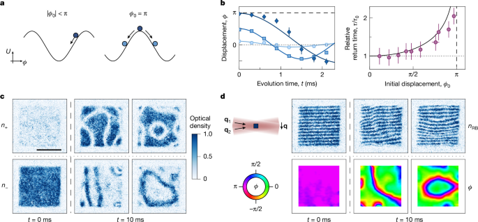
a, We study the dynamics following a large initial phase displacement ϕ0. For ∣ϕ0∣ < π, the plasma-oscillation period is ϕ0-dependent owing to the concavity of U(ϕ). For ϕ0 = π, different regions of the system may eventually settle to different potential minima, which results in domain walls across which ϕ winds by 2π. b, Large-amplitude oscillations. Left: for different ϕ0, the system takes different time, τ, to return to ϕ = 0. Solid lines show sinusoidal fits; for large ϕ0, the oscillation is visibly anharmonic. Each data point is based on five independent experimental runs, and the error bars show the s.e.m. Right: τ/τ0 versus ϕ0; here τ0 = π/(2ωp) is the ϕ0-independent perturbative result. The solid line is the prediction based on the pendulum model. The errors in τ correspond to half of the spacing between the sampled t values. Here, Z0 = 0.31, Ω/(2π) = 74 Hz and μs/(ħΩ) ≈ 11. c,d, Domain walls. The system is prepared at ϕ ≈ π at t = 0, and allowed to relax for 10 ms, corresponding to approximately 7τ0; here Z0 = 0.53, Ω/(2π) = 22 Hz and μs/(ħΩ) ≈ 39. Scale bar, 20 μm. In c, we show examples of domain walls seen in n+ and n− images, where they appear as, respectively, low- and high-density lines; each image shows an independent realization. In d, we show phase maps that reveal the 2π phase winding at domain walls. We interfere the two spin states using a pair of Raman–Bragg laser beams with wavevectors q1,2, and the imaged density distribution, nRB, shows modulations \(\propto \cos ({\bf{q}}\cdot {\bf{r}}+\phi )\), where q = q1 − q2 and r = (x, y). From such fringe patterns we reconstruct the phase maps shown in the bottom panels (see text for details).
For ∣ϕ0∣ < π, we observe the anharmonic nature of the sine-Gordon potential, \(U(\phi )\propto -\cos (\phi )\), by measuring the time, τ, it takes the system to return from ϕ0 to ϕ = 0 (Fig. 5b). Here, we extract \(\phi =\arctan (Y/X)\), where Y and X are the separately measured projections of the global Bloch vector. In the perturbative regime, U(ϕ) is approximately harmonic and τ ≈ π/(2ωp) is independent of ϕ0. However, as ϕ0 → π, the concavity of U becomes increasingly relevant and τ grows, in analogy with a mechanical pendulum with a large initial angular displacement (solid line in Fig. 5b, right). At longer times these oscillations damp out, and this damping is accompanied by an emergence of spatial structures corresponding to k > 0 excitations (Extended Data Fig. 2).
For ϕ0 = π, different regions of the system may settle into different potential minima, leading to the formation of domain walls across which ϕ rapidly winds by 2π. We observe such walls in most experimental realizations, with their spatial patterns varying randomly shot to shot (Fig. 5c,d).
In the images of n+ and n− (Fig. 5c), the walls appear as lines of low and high density, respectively. Here we show images from different experimental realizations, but note that if we image both n+ and n− in the same experimental run, we see that they are complementary (Extended Data Fig. 3).
In Fig. 5d, we explicitly demonstrate the 2π phase winding across the domain walls. Here, just before imaging the \(|\uparrow \rangle \) component, we perform a fast (approximately 6 μs) π/2 spin rotation using a resonant two-photon Raman–Bragg coupling (see cartoon) instead of a radio-frequency field. Compared with the radio-frequency field that has a spatially uniform phase across the cloud, the Raman–Bragg coupling leads to a complex Ω with a spatially varying phase q ⋅ r; here r = (x, y) and q = q1 − q2, where q1,2 are the wavevectors of the two laser beams. In the Bloch-sphere picture, the Raman–Bragg Rabi vector always lies in the equatorial plane, but its orientation varies along the direction defined by q. Consequently, the imaged density nRB(x, y) shows modulations \(\propto \cos ({\bf{q}}\cdot {\bf{r}}+\phi )\). For a spatially uniform ϕ, this is a pattern of straight parallel fringes with period 2π/q ≈ 2.51 μm, whereas spatial variations of ϕ(x, y) lead to fringe deformations. In particular, a domain wall perpendicular to q changes the fringe spacing, whereas a wall parallel to q shifts the fringe phase by 2π. In Fig. 5d, we show both the straight fringes observed at t = 0 ms and two examples of domain walls observed after 10 ms of relaxation; the bottom panels show the reconstructed phase maps (see Extended Data Fig. 4 for more details).
The characteristic width, w, of an equilibrium domain wall is set by the competition between the potential energy per unit length, ∝ ħΩ ⋅ nw, and the corresponding kinetic energy, ∝ ħ2/(2mw2) ⋅ nw. Similarly to the oscillator length in a quantum harmonic oscillator, this competition gives w = ƛ = \({\xi }_{{\rm{M}}}=\sqrt{\hbar /(2m\varOmega )}\).
In Fig. 6a, we extract the domain-wall widths from both the n± images and the phase maps. In all cases, one-dimensional cuts perpendicular to the walls are fitted well by the theoretically predicted10 forms n±(z) = n0 ± n1sech2(z/w) and ϕ(z) = 4arctan[exp(z/w)]; here, z is the coordinate perpendicular to a wall centred at z = 0, and n0, n1 and w are fit parameters. The extracted values of w have a wide distribution (see histograms), probably because our domain walls are excited, but the three mean values are (within one standard deviation) consistent with each other and with the theoretically predicted w, indicated on the histograms by the dashed lines; it is noted that here we include an 8% correction to the predicted w due to our non-zero Z0 (Methods).
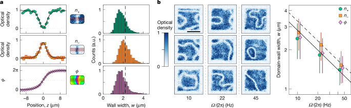
a, For the experimental protocol as in Fig. 5, we extract the wall widths, w, from n+ and n− images, such as shown in Fig. 5c, and the phase maps, such as shown in Fig. 5d. We fit cuts perpendicular to the walls to the theoretically expected profiles (solid lines, see text). The histograms show width distributions based on >100 experimental images, and the dashed lines indicate the theoretically predicted w. b, The effect of changing Ω on the domain-wall width. Here the experimental protocol is the same, except that for the last 2 ms of relaxation we jump Ω/(2π) from 22 Hz to either 10 Hz or 45 Hz. The representative n+ images show an increase of the wall widths in the former case and decrease in the latter. Scale bar, 20 μm. The summary of the extracted mean widths is consistent with the expected trend \(w\propto 1/\sqrt{\varOmega }\). The dashed line shows the theoretically predicted w, including an 8% correction due to our non-zero Z0 (Methods). The solid line shows the same trend with systematically 15% lower values. The error bars show the standard deviations of the w distributions. The different symbols corresponding to the same Ω are slightly offset horizontally for clarity.
Finally, in Fig. 6b, we show that the characteristic wall width responds to changes in Ω. Here we initiate the system dynamics as in Fig. 5c, but quench Ω either down or up for the last 2 ms of relaxation. In the representative n+ images, one can see the systematic change in the wall widths, and the widths extracted as in Fig. 6a are consistent with the expected trend \(w\propto 1/\sqrt{\varOmega }\).
To conclude, we have established a versatile analogue simulator for self-interacting relativistic quantum fields with a tunable mass in 2 + 1 dimensions, and observed non-perturbative phenomena that point the way to many future studies. The damping of the global ϕ oscillations, accompanied by an emergence of spatial structures (k > 0 excitations), is expected to be analogous to cosmological preheating and reheating11,12. The π phase jump that places the field at the top of the sine-Gordon potential initiates dynamics associated with a quench through a discrete symmetry-breaking phase transition (with the energy minima changing from ϕ = π to ϕ = 0 and 2π). Generalizing the π phase jump to a ramp of Ω from a positive to a negative value, one can study the associated Kibble–Zurek mechanism50, linked to the formation of topological defects such as cosmic strings and domain walls13,14. Studies of domain-wall networks could provide insights into cosmological dark-matter production in axion scenarios51,52 and gravitational-wave signals in a broad family of particle-physics models53. In this context, a particularly interesting possibility is to use vector light shifts to deterministically imprint specific initial domain-wall configurations and study their subsequent dynamics, including their relaxation and decay54,55. Finally, using Floquet engineering to stabilize the system at ϕ = π would enable studies of false-vacuum decay15,16,41,42 in a relativistic, cosmologically relevant setting17,18,19.